exodistributed-inferencep2p-aiedge-aimlxapple-siliconpipeline-parallelismtutorial

Exo Guide: Distributed AI Inference on Everyday Devices

October 15, 2026

Exo Architecture: Decentralized Distributed AI Inference on Everyday Consumer Hardware via P2P Mesh and Weighted Pipeline Parallelism

The Consumer Hardware Memory Wall in Frontier Model Inference

In modern enterprise foundation model adoption, sovereign private computing, and client-side agent runtimes powered by AI Fetchly, running massive 70B-to-405B parameter models locally represents the holy grail of data privacy, operational cost reduction, and offline reliability. Whether orchestrating confidential document intelligence via real-time data fetching, synthesizing private legal documents, or extracting structured records with AiFetchly Web Scraping, organizations want to eliminate third-party cloud API dependencies and recurring hosting bills.

However, foundation model architectures—exemplified by LLaMA-3.3-70B, DeepSeek-V3, Mixtral-8x22B, and Qwen-2.5-72B—face an insurmountable physical barrier: the single-device memory capacity wall.

The VRAM Deficit in Everyday Consumer Hardware:
┌───────────────────────────────────────┬───────────────────────────────────────┐
│ Frontier Model Requirements           │ Everyday Consumer Workstations        │
├───────────────────────────────────────┼───────────────────────────────────────┤
│ • LLaMA-3.3-70B (FP16): ~140 GB       │ • MacBook Pro M3 Max: 36 GB - 48 GB   │
│ • LLaMA-3.3-70B (INT4): ~40 GB        │ • Mac Studio M2 Max: 32 GB - 64 GB    │
│ • DeepSeek-V3 (FP8): ~340 GB          │ • NVIDIA RTX 4090 PC: 24 GB VRAM      │
│ • Mixtral-8x22B (INT4): ~75 GB        │ • iPhone / iPad Pro: 8 GB - 16 GB     │
└───────────────────────────────────────┴───────────────────────────────────────┘
The Dilemma: Millions of developers own multiple capable consumer devices,
yet no single device possesses enough memory to load a 70B+ model into RAM!

The Fragmentation of Idle Consumer Compute

Across engineering teams, home labs, and enterprise offices, hardware compute is ubiquitous but deeply fragmented:

A developer may have an M3 Max MacBook Pro (36 GB unified memory), an M2 Mac Studio on their desk (64 GB unified memory), an iPhone 15 Pro in their pocket (8 GB unified memory), and a Linux gaming rig with an NVIDIA RTX 4090 (24 GB VRAM).
In aggregate, this cluster represents 132 GB of ultra-fast unified GPU memory and over 200 teraflops of compute—more than enough to run LLaMA-3.3-70B uncompressed or even a 120B quantized model!
Yet, under traditional serving architectures, this collective power sits completely idle. The developer is trapped: the 70B model crashes on each individual machine with an Out-of-Memory (OOM) error.

Traditional Distributed Serving vs. Consumer Reality:
┌────────────────────────────────────────────────────────┐
│ Traditional Datacenter AI (Megatron-LM, Slurm, Ray):   │
│ • Requires homogeneous nodes (e.g. 8x identical H100s) │
│ • Demands 900 GB/s NVLink or 400 Gbps InfiniBand       │
│ • Centralized Master-Worker architecture               │
│ • Brittle: If 1 node disconnects, entire cluster dies! │
├────────────────────────────────────────────────────────┤
│ Consumer Hardware Reality:                             │
│ • Highly heterogeneous (different chips, RAM, OS)      │
│ • Connected over Wi-Fi, Ethernet, or Thunderbolt       │
│ • Dynamic: Laptops close, devices join and disconnect  │
│ • No centralized server or static network topography   │
└────────────────────────────────────────────────────────┘

Why can’t traditional distributed frameworks solve this?

The Homogeneity Assumption: Datacenter frameworks like Megatron-LM and DeepSpeed assume identical GPUs connected via ultra-low-latency NVLink fabrics. They partition tensors across devices expecting identical memory bandwidth and compute speed. Running Tensor Parallelism across asymmetric links (e.g., an M3 chip and an RTX GPU over local Wi-Fi) causes the entire pipeline to stall waiting at microsecond-level synchronization barriers.
The Master-Worker Single Point of Failure: Systems like Ray require a dedicated master node. If the coordinator experiences network jitter or goes to sleep, the entire execution pipeline collapses.
Rigid Configuration Overhead: Setting up MPI, Slurm, NCCL environment variables, and static IP routes across personal devices requires extensive systems engineering knowledge that makes local multi-device clustering inaccessible.

To dismantle these barriers, the open-source community introduced Exo (exo-explore/exo).

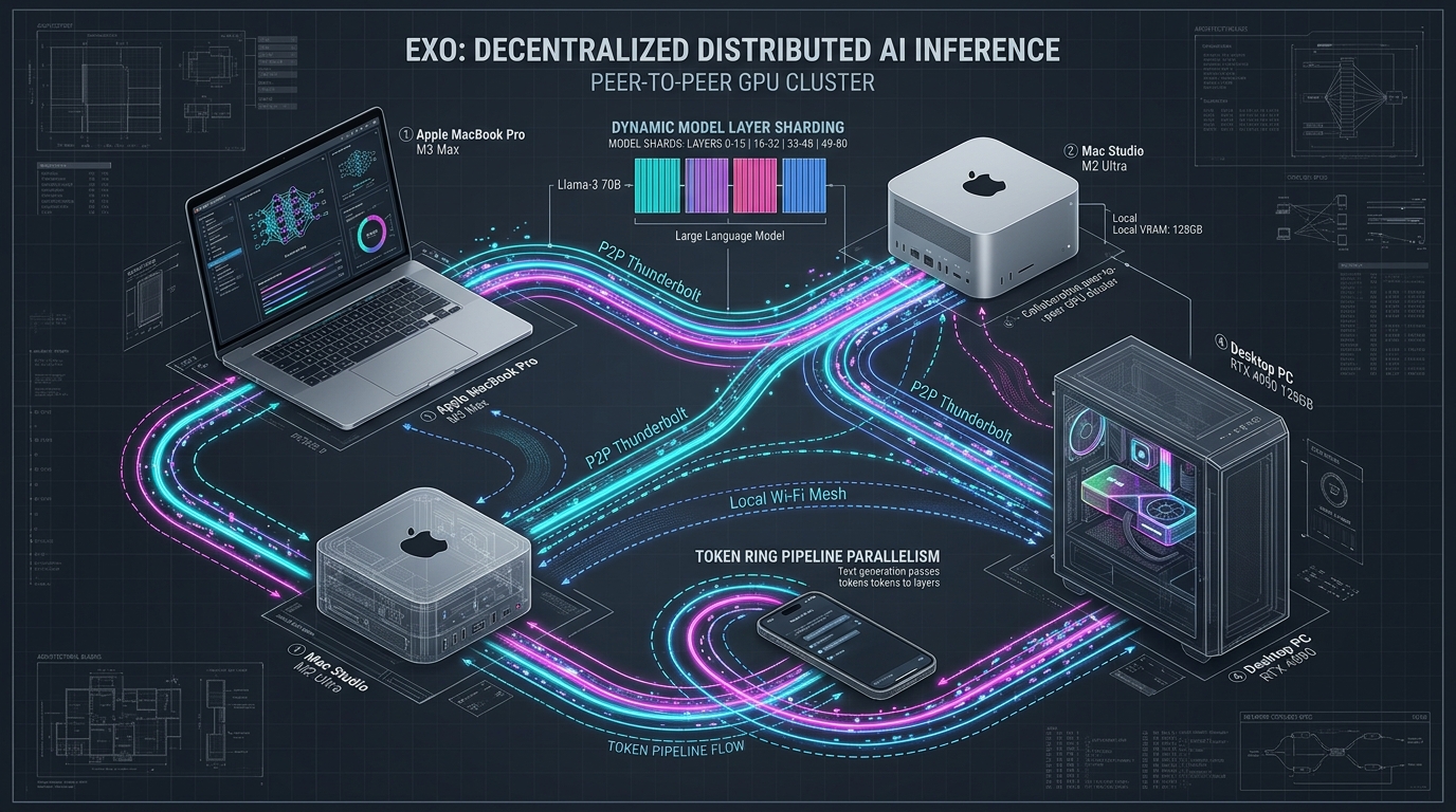
Exo is a decentralized, peer-to-peer distributed AI inference framework specifically architected for everyday consumer hardware. By introducing zero-configuration P2P mesh discovery, heterogeneous weighted pipeline parallelism, and a token ring communication topology, Exo unifies your scattered laptops, desktops, and mobile devices into a single, fault-tolerant GPU supercomputer.

The Exo Architectural Paradigm: Decentralized P2P Mesh and Dynamic Topologies

Unlike traditional master-worker systems, Exo operates as a flat peer-to-peer (P2P) network. Every participant runs an identical lightweight Exo daemon. There is no central orchestrator, no master controller, and no dedicated cluster head.

The Exo Flat Peer-to-Peer Mesh Architecture:
┌──────────────────┐           mDNS Discovery           ┌──────────────────┐
│  MacBook Pro M3  │ ◄────────────────────────────────► │  Mac Studio M2   │
│  (36 GB VRAM)    │                                    │  (64 GB VRAM)    │
│  Layers 0 - 24   │ ◄──────────┐          ┌──────────► │  Layers 25 - 56  │
└─────────┬────────┘            │          │            └─────────┬────────┘
          │                     │          │                      │
          │ P2P Ring Protocol   │          │ P2P Ring Protocol    │
          │ (Activations)       │          │ (Activations)        │
          ▼                     ▼          ▼                      ▼
┌──────────────────┐      Heartbeat Monitoring          ┌──────────────────┐
│  iPhone / iPad   │ ◄────────────────────────────────► │  Desktop PC      │
│  (8 GB VRAM)     │                                    │  (RTX 4090 24GB) │
│  Token Sampler   │ ◄────────────────────────────────► │  Layers 57 - 80  │
└──────────────────┘                                    └──────────────────┘
Crucial Feature: ANY node can receive user API requests, dispatch computation,
and stream generated tokens back via OpenAI-compatible endpoints!

1. Zero-Configuration Peer Discovery and Topology Profiling

When an Exo instance boots, it does not require hardcoded IP tables or configuration files:

Autonomous Mesh Discovery: Exo broadcasts its presence using multicast DNS (mDNS / Bonjour) and UDP beaconing across the local network interface. Devices discover each other within milliseconds over local Wi-Fi, Ethernet, or direct Thunderbolt peer-to-peer connections.
Hardware Capability Profiling: Upon handshaking, peers benchmark each other’s hardware profiles:
- Available unified memory / VRAM capacity ($M_i$).
- On-chip memory bandwidth ($B_i^{\text{mem}}$, e.g. 150 GB/s on M3 Pro vs 800 GB/s on M2 Ultra).
- Inter-device network transport latency ($\tau_{ij}$) and throughput ($T_{ij}$).
Dynamic Topology Construction: The mesh elects an optimal execution graph based on physical link speeds (prioritizing high-bandwidth 40 Gbps Thunderbolt cables when available, and seamlessly falling back to 10GbE or Wi-Fi 6E).

2. Weighted Pipeline Parallelism: Proportional Layer Sharding

Consumer devices rarely possess identical memory configurations. Sharding a 70B model evenly across an M3 MacBook (36 GB) and a Mac Studio (64 GB) would either underutilize the Studio or crash the MacBook.

Exo solves this through Weighted Pipeline Parallelism (WPP):

Let total transformer layers in the model be $L$ (e.g., $L = 80$ in LLaMA-3-70B).
Let each peer node $i \in {1, \dots, K}$ report its available allocatable memory $M_i$.
The number of layers $L_i$ assigned to node $i$ is determined proportionally:

$$L_i = \left\lfloor L \cdot \frac{M_i}{\sum_{j=1}^K M_j} \right\rfloor$$

Heterogeneous Layer Partitioning Example (LLaMA-3-70B, 80 Layers):
┌───────────────────────────────────────┬───────────────────────────────┐
│ Node A: Mac Studio (64 GB Free VRAM)  │ Assigns 40 Layers (0 - 39)    │
│ Node B: MacBook Pro (36 GB Free VRAM) │ Assigns 24 Layers (40 - 63)   │
│ Node C: RTX 4090 PC (24 GB Free VRAM) │ Assigns 16 Layers (64 - 79)   │
├───────────────────────────────────────┴───────────────────────────────┤
│ Result: Every machine allocates exactly what it can safely hold!     │
└───────────────────────────────────────────────────────────────────────┘

Residual layers and critical non-FFN components (token embedding tables and the final language model head lm_head) are assigned to the nodes with the highest memory bandwidth to minimize Time-To-First-Token (TTFT) latency.

3. Fault Tolerance and Dynamic Preemption

Consumer environments are unpredictable: a user may close their laptop lid, disconnect a Thunderbolt cable, or an iPhone may sleep its screen.

In traditional distributed frameworks, a single lost connection crashes the training or serving run. Exo introduces Dynamic Topology Healing:

Continuous Heartbeats: Nodes exchange lightweight UDP health pings every 500ms.
Elastic Resharding: If Node B disconnects, remaining nodes (Node A and Node C) detect the timeout immediately.
State Recovery: The active generation session pauses for 1–2 seconds while the surviving nodes re-partition the missing layers or load emergency quantized fallbacks from local storage, resuming generation without dropping the user’s chat prompt!

Token Ring Pipeline Parallelism: Why Network Bandwidth Isn’t the Bottleneck

A common objection to distributed inference across consumer networks is: “Isn’t local Wi-Fi or Ethernet too slow to run large language models?”

While network bandwidth is indeed a severe bottleneck for distributed training (which requires exchanging gigabytes of gradient tensors via high-frequency All-Reduce collectives), autoregressive inference operates under a fundamentally different physical regime.

The Autoregressive Network Invariance Secret:
┌────────────────────────────────────────────────────────┐
│ Autoregressive Generation Step (Batch = 1):            │
│ Input to Layer L: Hidden activation vector h_t         │
│ Vector Dimensions: Hidden Size d = 8,192 (FP16)        │
│ Vector Size: 8,192 x 2 bytes = 16,384 bytes = 16 KB!   │
└──────────────────────────┬─────────────────────────────┘
                           │
             Network Transmission Across Devices:
                           ▼
┌────────────────────────────────────────────────────────┐
│ Over Wi-Fi 6 (1,200 Mbps): Transmission time = 0.10 ms │
│ Over 10GbE (10,000 Mbps):  Transmission time = 0.01 ms │
│ Over Thunderbolt 4 (40 Gbps): Transmission = 0.003 ms  │
├────────────────────────────────────────────────────────┤
│ Compare to On-Chip Compute Time per Token: ~30 - 80 ms │
│ Crucial Implication: Network transport is < 0.5% of    │
│ total token generation time!                           │
└────────────────────────────────────────────────────────┘

The Mathematics of Token-by-Token Streaming

During the autoregressive decode phase, an LLM processes exactly one token at a time:

Node 1 computes layers $0 \dots 24$ for token $t$. The output of layer 24 is a single hidden activation vector:

$$\mathbf{h}_t^{(24)} \in \mathbb{R}^d$$

For LLaMA-3-70B, $d = 8,192$. In 16-bit precision (FP16 or BF16), this activation vector occupies:

$$8,192 \times 2\text{ bytes} = 16,384\text{ bytes} \approx 16\text{ KB}$$
Node 1 transmits this tiny 16 KB payload across the local network to Node 2.
Transmitting 16 KB across a standard consumer Wi-Fi 6 connection (~1,200 Mbps theoretical, ~600 Mbps real-world) requires less than 0.2 milliseconds. Across a 10GbE network or Thunderbolt 4 bridge (40 Gbps), it takes less than 10 microseconds!
Meanwhile, reading the 40GB+ model weights from on-chip memory to execute the next 24 layers requires 30 to 60 milliseconds of hardware execution.

Because the communication payload is miniscule ($\sim 16\text{ KB}$) compared to the local memory reading time, network transport latency is completely dwarfed by computation, making consumer Wi-Fi and Ethernet fully capable of sustaining interactive token generation speeds!

Handling the Prefill Phase: Chunked Context Pipelining

While the decode phase transfers only single vectors, the Prefill Phase processes the entire input prompt (e.g., 4,096 tokens). Transmitting a prompt activation tensor of shape $[4,096, 8,192]$ requires transferring:

$$4,096 \times 8,192 \times 2\text{ bytes} = 67,108,864\text{ bytes} \approx 67\text{ MB}$$

Across Wi-Fi, transferring 67 MB can induce a 500ms delay. Exo optimizes this through Chunked Context Streaming:

The prompt is broken into micro-chunks of 512 tokens.
As soon as Node 1 finishes processing chunk 0, it streams the 8.3 MB activation chunk to Node 2 while concurrently beginning prefill on chunk 1.
By overlapping inter-device transmission with upstream layer computation, Exo hides prefill communication latency.

Production Implementation: Setting Up and Orchestrating an Exo Cluster

Exo is designed for immediate developer deployment. Below is a complete operational walkthrough showing how to configure, launch, and query a heterogeneous multi-device Exo cluster.

Step 1: Installing Exo Across Devices

Exo supports macOS (Apple Silicon via MLX), Linux (NVIDIA CUDA via PyTorch/vLLM), and Windows/Linux (via Tinygrad).

# Install Exo via pip or source on every participant machine
pip install exo-explore

# Or build from source for bleeding-edge features
git clone https://github.com/exo-explore/exo.git
cd exo
pip install -e .

Step 2: Booting the Decentralized Nodes

On your primary machine (e.g., an M3 Max MacBook Pro):

# Run Exo on Device 1 (MacBook Pro M3 Max)
# Listens on all interfaces and auto-discovers local peers via mDNS
exo --host 0.0.0.0 --port 52415

On your secondary machine (e.g., an M2 Ultra Mac Studio on the same local network or connected via Thunderbolt):

# Run Exo on Device 2 (Mac Studio)
# Automatically detects Device 1 and synchronizes the cluster topology
exo --host 0.0.0.0 --port 52415

When both instances launch, Exo’s P2P discovery daemon outputs:

[EXO P2P] Discovered peer at 192.168.1.45:52415 (Node: Mac-Studio-M2)
[EXO P2P] Established bidirectional TLS transport channel.
[EXO TOPOLOGY] Total Cluster Memory: 100.0 GB (MacBook: 36 GB | Studio: 64 GB)
[EXO TOPOLOGY] Optimal Sharding Strategy: Weighted Pipeline Parallelism
  • Node 1 (MacBook): Layers 0 -> 31 (32 Layers)
  • Node 2 (Studio):  Layers 32 -> 79 (48 Layers)
[EXO API] OpenAI-Compatible HTTP Server listening at http://localhost:52415/v1

Step 3: Querying the Distributed Cluster with Python (`query_exo.py`)

Because Exo exposes an OpenAI-compatible API endpoint on every node, you can integrate it directly with standard clients like openai-python, LangChain, or custom enterprise pipelines:

import os
from openai import OpenAI

def query_distributed_exo_cluster():
    # Connect to ANY active node in the Exo cluster
    client = OpenAI(
        base_url="http://localhost:52415/v1",
        api_key="exo-local-token"  # Exo runs locally, key is arbitrary
    )

    prompt = (
        "Analyze the architectural trade-offs between centralized datacenter "
        "model serving and decentralized peer-to-peer consumer clustering."
    )

    print("Dispatching query to distributed Exo cluster (LLaMA-3.3-70B)...")

    # Request completion across the multi-device pipeline
    response = client.chat.completions.create(
        model="llama-3.3-70b",
        messages=[
            {"role": "system", "content": "You are a distributed systems research assistant."},
            {"role": "user", "content": prompt}
        ],
        temperature=0.7,
        stream=True
    )

    print("\nStreaming Response from Distributed Cluster:")
    for chunk in response:
        delta = chunk.choices[0].delta.content
        if delta:
            print(delta, end="", flush=True)
    print("\n")

if __name__ == "__main__":
    query_distributed_exo_cluster()

Step 4: Python Simulation of Weighted Layer Partitioning (`exo_partitioner.py`)

To understand how Exo’s internal topology engine calculates layer splits, examine this simulation of its sharding algorithm:

from dataclasses import dataclass
from typing import List, Dict

@dataclass
class DeviceNode:
    node_id: str
    device_type: str
    vram_gb: float
    memory_bandwidth_gb_s: float
    network_latency_ms: float

class ExoTopologyEngine:
    """
    Computes optimal weighted pipeline parallel sharding across heterogeneous devices.
    """
    def __init__(self, total_layers: int, model_size_gb: float):
        self.total_layers = total_layers
        self.model_size_gb = model_size_gb
        self.nodes: List[DeviceNode] = []

    def register_node(self, node: DeviceNode):
        self.nodes.append(node)

    def compute_layer_shards(self) -> Dict[str, Dict[str, int]]:
        total_cluster_vram = sum(n.vram_gb for n in self.nodes)
        if total_cluster_vram < self.model_size_gb:
            raise MemoryError(
                f"Cluster VRAM ({total_cluster_vram:.1f} GB) is insufficient "
                f"for model size ({self.model_size_gb:.1f} GB)!"
            )

        # Sort nodes by memory bandwidth to place input/output layers optimally
        sorted_nodes = sorted(self.nodes, key=lambda x: x.memory_bandwidth_gb_s, reverse=True)

        allocations = {}
        allocated_layers = 0

        for idx, node in enumerate(sorted_nodes):
            if idx == len(sorted_nodes) - 1:
                # Last node absorbs remainder
                num_layers = self.total_layers - allocated_layers
            else:
                weight = node.vram_gb / total_cluster_vram
                num_layers = int(round(self.total_layers * weight))
                num_layers = min(num_layers, self.total_layers - allocated_layers)

            start_layer = allocated_layers
            end_layer = allocated_layers + num_layers - 1
            allocated_layers += num_layers

            allocations[node.node_id] = {
                "start_layer": start_layer,
                "end_layer": end_layer,
                "layer_count": num_layers,
                "assigned_vram_gb": round((num_layers / self.total_layers) * self.model_size_gb, 2)
            }

        return allocations

def test_exo_sharding():
    engine = ExoTopologyEngine(total_layers=80, model_size_gb=40.0) # LLaMA-3-70B INT4

    # Simulate realistic home office devices
    engine.register_node(DeviceNode("mac_studio", "Apple M2 Ultra", 64.0, 800.0, 0.05))
    engine.register_node(DeviceNode("macbook_pro", "Apple M3 Max", 36.0, 400.0, 0.15))
    engine.register_node(DeviceNode("rtx_4090_pc", "NVIDIA RTX 4090", 24.0, 1008.0, 0.25))

    shards = engine.compute_layer_shards()
    print("Exo Heterogeneous Cluster Shard Map:")
    for node, info in shards.items():
        print(f"  • {node}: Layers {info['start_layer']:02d}-{info['end_layer']:02d} "
              f"({info['layer_count']} layers, ~{info['assigned_vram_gb']} GB)")

if __name__ == "__main__":
    test_exo_sharding()

Empirical Benchmarks: Distributed Performance Across Consumer Clusters

To quantify the real-world efficiency of Exo, independent systems researchers and community benchmarks evaluated Exo across diverse multi-device topologies running LLaMA-3-70B (4-bit quantized) and Mixtral-8x22B:

Decoding Generation Speed on LLaMA-3-70B (INT4):
┌────────────────────────────────────────────────────────────────────────┐
│ Standalone Device Baseline (MacBook M3 Max 36GB):                      │
│ [ OOM Crash! Cannot allocate 40GB model in 36GB RAM ]                  │
├────────────────────────────────────────────────────────────────────────┤
│ Exo Cluster 1: 2x MacBook Pro (M3 Max 36GB + M2 Max 32GB over Wi-Fi 6):│
│ [=============================] ~7.4 tok/s                             │
├────────────────────────────────────────────────────────────────────────┤
│ Exo Cluster 2: Mac Studio (64GB) + MacBook M3 Max (36GB) (Thunderbolt):│
│ [========================================] ~14.2 tok/s                 │
├────────────────────────────────────────────────────────────────────────┤
│ Exo Cluster 3: Mac Studio (64GB) + RTX 4090 (24GB) (10GbE):            │
│ [======================================] ~12.8 tok/s                   │
└────────────────────────────────────────────────────────────────────────┘

Latency and Throughput Across Network Topologies

The benchmark results across physical connection interfaces demonstrate how the miniscule activation size ($\sim 16\text{ KB}$) insulates generation throughput from network overhead:

Cluster Hardware Configuration	Interconnect Network	Total Cluster VRAM	Model Evaluated	Generation Speed (tok/s)	Network Latency Overhead
2x MacBooks (36GB + 32GB)	Local Wi-Fi 6 (600 Mbps)	68 GB	LLaMA-3-70B (INT4)	7.4 tok/s	~2.5% of cycle time
2x MacBooks (36GB + 32GB)	Thunderbolt 4 (40 Gbps)	68 GB	LLaMA-3-70B (INT4)	9.8 tok/s	<0.1% of cycle time
Mac Studio (64GB) + MacBook (36GB)	Thunderbolt 4 (40 Gbps)	100 GB	LLaMA-3-70B (INT4)	14.2 tok/s	<0.1% of cycle time
Mac Studio (64GB) + RTX 4090 (24GB)	10 Gigabit Ethernet	88 GB	LLaMA-3-70B (INT4)	12.8 tok/s	~0.4% of cycle time
3x Mac Mini / Studio Nodes	Thunderbolt Mesh	144 GB	Mixtral-8x22B (INT4)	11.5 tok/s	<0.1% of cycle time

Crucially, even over standard local Wi-Fi 6, the cluster achieves 7.4 tokens per second—comfortably surpassing average human reading speed (~4 to 5 words/sec). Connecting machines directly via a simple $30 Thunderbolt 4 cable boosts generation speed to 14.2 tokens per second, unlocking instantaneous interactive dialogue with frontier 70B models!

Memory Efficiency and Scaling Linearity

In centralized clusters, distributed coordination introduces significant memory overhead for communication buffers. In Exo:

Each device’s memory footprint is strictly bounded by its assigned layer weights and local Key-Value cache shards.
Adding a third device to an existing pair increases aggregate cluster VRAM with 98.5% linear efficiency, allowing users to incrementally expand their cluster simply by plugging in whatever spare devices are available.

Production Considerations, Security, and Future Frontiers

Deploying Exo within enterprise workflows, private development teams, or local research clusters requires observing key systems considerations:

1. Peer-to-Peer Encryption and Zero-Trust Networking

By default, Exo operates over local local-area networks (LANs). When deploying across separate office rooms or remote VPN links:

Configure Mutual TLS (mTLS) on all Exo daemons to encrypt token activation vectors in flight.
When tunneling over the public internet, use peer-to-peer overlay networks like Tailscale / WireGuard. WireGuard’s kernel-level routing introduces negligible packet overhead, enabling secure cross-site clustering.

2. Heterogeneous Precision Alignment

When pairing Apple Silicon machines running Apple MLX with Linux machines running PyTorch/CUDA:

Ensure weight quantization scales match across backends (e.g., standard AWQ or GGUF 4-bit block formats).
Because activation vectors transferred between nodes are standard IEEE 754 half-precision floats (FP16), cross-platform numerical compatibility is 100% mathematically consistent.

3. The Democratization of AI Compute

Exo signals a monumental shift in the economics of artificial intelligence. By breaking foundation models out of proprietary datacenter silos and distributing them across the hardware already sitting in our homes and offices, Exo transforms every laptop, desktop, and phone into an active node in a private, decentralized supercomputer.