DualPipe: Bidirectional Pipeline Parallelism Guide
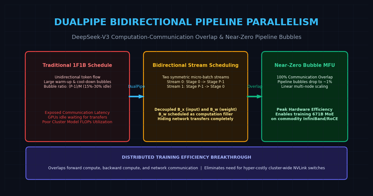
The Problem: The Pipeline Bubble and the Communication Bottleneck
When scaling frontier foundation models beyond hundreds of billions of parameters (such as DeepSeek-V3’s 671B architecture), the model’s layers exceed the physical memory capacity of any single 8-GPU node. To distribute training, engineering teams partition model layers across $P$ sequential pipeline stages using Pipeline Parallelism (PP).
In standard pipeline parallelism, training data is divided into $M$ discrete micro-batches. In the classical 1F1B (One Forward, One Backward) scheduling scheme popularized by Megatron-LM, each pipeline stage alternates between executing one forward micro-batch and one backward micro-batch.
However, standard 1F1B introduces two severe structural bottlenecks that cripple hardware efficiency at scale:
1. The Pipeline Bubble (Idle GPU Hardware)
Because micro-batches must traverse stages sequentially (Stage $0 \to 1 \to \dots \to P-1$), downstream GPUs sit completely idle during the initial “warm-up” phase waiting for activations to arrive. Conversely, upstream GPUs sit idle during the “cool-down” phase waiting for backward gradients to propagate back.
The theoretical bubble fraction in standard 1F1B is governed by:
$$F_{\text{bubble}} = \frac{P - 1}{M}$$
To shrink the bubble fraction to an acceptable level (e.g., $<10%$), cluster operators must inflate $M$ relative to $P$. However, increasing $M$ causes peak activation memory to skyrocket—demanding that GPUs retain up to $P$ micro-batches of uncompressed forward activations simultaneously, frequently triggering Out-of-Memory (OOM) failures.
2. Exposed Inter-Node Communication Latency
In standard pipeline schedules, computation and inter-node network communication occur synchronously:
- When Stage $i$ completes its forward pass, it must transmit activation tensors across InfiniBand or RoCE network switches to Stage $i+1$.
- During backward propagation, Stage $i+1$ must transmit activation gradients back to Stage $i$.
Because inter-node network bandwidth (typically 400 Gbps to 800 Gbps) is orders of magnitude slower than intra-node NVLink interconnects (up to 3.2 Tbps), GPUs spend 20% to 35% of their total cycle time idling while awaiting network packet exchanges.
The Solution: DeepSeek-V3 DualPipe
Introduced in the DeepSeek-V3 technical report and open-sourced in the deepseek-ai/DualPipe repository, DualPipe is a bidirectional pipeline parallelism algorithm designed to eliminate both the pipeline bubble and exposed communication latency.
Rather than pumping micro-batches unidirectionally across the cluster, DualPipe reorganizes cluster execution around two foundational architectural principles:
- Bidirectional Micro-Batch Streams: Two symmetric streams of micro-batches (Stream 0 and Stream 1) are injected into the pipeline simultaneously from opposite ends.
- Decoupling Backward Input ($B_x$) from Backward Weight ($B_w$): Splitting the backward execution pass into activation gradient computation and parameter weight gradient computation.
The Three Pipeline Operators in DualPipe
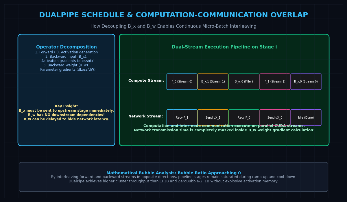
In classical deep learning frameworks, the backward pass is treated as a monolithic operator $B$. DualPipe breaks execution into three distinct phases:
- Forward ($F$): Generates layer activations and produces output activations for the subsequent stage.
- Backward Input ($B_x$): Computes activation gradients $\nabla_{\mathbf{x}} = \frac{\partial \mathcal{L}}{\partial \mathbf{x}}$ needed by the upstream stage to continue backpropagation.
- Backward Weight ($B_w$): Computes parameter gradients $\nabla_{\mathbf{W}} = \frac{\partial \mathcal{L}}{\partial \mathbf{W}}$ to update local layer weights.
Crucially, $B_x$ has strict dependencies (the upstream stage cannot proceed without $\nabla_{\mathbf{x}}$), while $B_w$ has zero downstream dependencies—its parameter gradients accumulate locally inside the GPU’s own optimizer buffer.
DualPipe exploits this mathematical reality by scheduling $B_w$ opportunistically as computation filler to completely mask inter-node network communication!
Key Architectural Mechanics
1. The Symmetric Bidirectional Schedule
In DualPipe, model layers are partitioned across $P$ physical stages:
- Forward Direction of Stream 0: Traverses from Stage $0 \longrightarrow \text{Stage } P-1$.
- Forward Direction of Stream 1: Traverses from Stage $P-1 \longrightarrow \text{Stage } 0$.
Because Stream 0 and Stream 1 enter the pipeline from opposite directions, when Stage 0 is warming up on Stream 0, Stage $P-1$ is warming up on Stream 1. The idle “bubbles” at the physical boundaries of the cluster are naturally occupied by the opposing stream.
2. Complete Computation-Communication Overlap
On any given GPU stage $i$, DualPipe launches separate CUDA execution streams for computation (Tensor Cores) and inter-node communication (NIC Direct Memory Access / NCCL):
- Stage $i$ completes Backward Input ($B_x$) on a micro-batch from Stream 0.
- The communication stream immediately initiates the non-blocking network transmission of $\nabla_{\mathbf{x}}$ to Stage $i-1$.
- Concurrently, the compute stream immediately begins executing the computationally heavy Backward Weight ($B_w$) operator for an earlier micro-batch.
- Because the time required to compute $B_w$ (GEMM) exceeds the transmission time of activation gradients over InfiniBand, the network latency is 100% hidden.
- By the time $B_w$ finishes, the network transfer is complete, and the next incoming micro-batch is already waiting in GPU SRAM.
3. Pipeline Bubble Ratio Comparison
Let $t_F, t_{B_x}, t_{B_w}$ denote the execution times of the respective operators, with $t_B = t_{B_x} + t_{B_w}$. In an ideal schedule where $t_F \approx t_{B_w}$:
$$\text{Bubble Ratio}_{\text{1F1B}} = \frac{P - 1}{M}$$
$$\text{Bubble Ratio}{\text{DualPipe}} \approx \frac{(P - 1) \cdot (t_F - t{B_w})}{M \cdot (t_F + t_{B_x} + t_{B_w})} \approx 0$$
Because $t_F$ and $t_{B_w}$ are mathematically balanced matrix multiplications, the numerator $(t_F - t_{B_w})$ approaches zero. The pipeline bubble virtually vanishes, enabling frontier clusters to achieve Model FLOPs Utilization (MFU) exceeding 55% across thousands of GPUs.
Distributed Pipeline Parallelism Comparison Matrix
| Architectural Dimension | Classical 1F1B | 1F1B-Interleaved | ZeroBubble (ZB-2F1B) | DeepSeek-V3 DualPipe |
|---|---|---|---|---|
| Pipeline Trajectory | Unidirectional ($0 \to P-1$) | Multiple virtual stages | Unidirectional ($0 \to P-1$) | Bidirectional symmetric ($0 \leftrightarrow P-1$) |
| Backward Pass Handling | Monolithic $B$ | Monolithic $B$ | Decoupled $B_x$ and $B_w$ | Decoupled $B_x$ and $B_w$ |
| Communication Overlap | Exposed to bubble | Exposed to bubble | Partial overlap | Full 100% overlap of $F, B_x$, and network |
| Activation Memory | $O(P)$ micro-batches | $O(P / v)$ micro-batches | $O(2P)$ micro-batches | $O(P)$ micro-batches (Symmetric) |
| Pipeline Bubble Fraction | High (15% – 30%) | Moderate (8% – 15%) | Low (4% – 8%) | Near-Zero (< 2%) |
| Network Fabric Demands | Requires ultra-fast NVLink | Requires high cross-mesh | High bandwidth | Resilient on commodity InfiniBand/RoCE |
Reference Implementation: DualPipe Schedule Simulator
Below is a complete, educational Python simulator demonstrating how DualPipe schedules bidirectional micro-batches, tracks operator dependencies ($F, B_x, B_w$), and verifies communication overlap.
from dataclasses import dataclass
from typing import List, Dict, Optional
import enum

class OpType(enum.Enum):
    FORWARD = "F"
    BACKWARD_INPUT = "B_x"
    BACKWARD_WEIGHT = "B_w"

@dataclass
class MicroBatchOp:
    stream_id: int          # 0 or 1
    mb_id: int              # Micro-batch index
    op_type: OpType
    stage_id: int
    duration: float = 1.0   # Normalized compute duration

class DualPipeStageSimulator:
    """
    Simulates the operator queue and execution sequence for a single pipeline stage.
    """
    def __init__(self, stage_id: int, num_stages: int):
        self.stage_id = stage_id
        self.num_stages = num_stages
        self.ready_queue: List[MicroBatchOp] = []
        self.execution_history: List[MicroBatchOp] = []
        self.activation_memory_count: int = 0
        self.peak_activation_memory: int = 0

    def add_operator(self, op: MicroBatchOp):
        self.ready_queue.append(op)

    def select_next_operator(self) -> Optional[MicroBatchOp]:
        """
        DualPipe Priority Selection Law:
        Priority: Backward Input (B_x) > Forward (F) > Backward Weight (B_w).
        B_x is prioritized to unblock upstream stages immediately.
        B_w is executed to fill compute gaps and hide communication.
        """
        if not self.ready_queue:
            return None

        # Sort based on priority
        priority = {OpType.BACKWARD_INPUT: 0, OpType.FORWARD: 1, OpType.BACKWARD_WEIGHT: 2}
        self.ready_queue.sort(key=lambda op: priority[op.op_type])

        selected = self.ready_queue.pop(0)

        # Track activation memory footprint
        if selected.op_type == OpType.FORWARD:
            self.activation_memory_count += 1
            self.peak_activation_memory = max(self.peak_activation_memory, self.activation_memory_count)
        elif selected.op_type == OpType.BACKWARD_INPUT:
            # Memory released once backward input finishes
            self.activation_memory_count = max(0, self.activation_memory_count - 1)

        self.execution_history.append(selected)
        return selected


# Demonstration: Scheduling on Stage 0 with 2 Bidirectional Streams
if __name__ == "__main__":
    stage = DualPipeStageSimulator(stage_id=0, num_stages=4)

    # Ingest simultaneous micro-batches from Stream 0 (forward) and Stream 1 (backward)
    ops = [
        MicroBatchOp(stream_id=0, mb_id=0, op_type=OpType.FORWARD, stage_id=0),
        MicroBatchOp(stream_id=0, mb_id=1, op_type=OpType.FORWARD, stage_id=0),
        MicroBatchOp(stream_id=1, mb_id=0, op_type=OpType.BACKWARD_INPUT, stage_id=0),
        MicroBatchOp(stream_id=1, mb_id=0, op_type=OpType.BACKWARD_WEIGHT, stage_id=0),
        MicroBatchOp(stream_id=0, mb_id=0, op_type=OpType.BACKWARD_INPUT, stage_id=0),
        MicroBatchOp(stream_id=0, mb_id=0, op_type=OpType.BACKWARD_WEIGHT, stage_id=0),
    ]

    for op in ops:
        stage.add_operator(op)

    print("--- Simulating DualPipe Operator Scheduling ---")
    step = 1
    while True:
        next_op = stage.select_next_operator()
        if not next_op:
            break
        print(f"Step {step:02d} | Executing: {next_op.op_type.value:<4} for Stream {next_op.stream_id} (MB {next_op.mb_id}) | Active Activations: {stage.activation_memory_count}")
        step += 1

print(f"\nScheduling complete. Peak activation memory held: {stage.peak_activation_memory} micro-batches") Production Scaling and Hardware Implications
DualPipe has fundamentally lowered the capital barrier for pretraining and fine-tuning multi-hundred-billion parameter models:
1. Breaking the Interconnect Monopoly
Historically, training massive foundation models required GPU supercomputers equipped with cluster-wide NVLink switches (such as NVIDIA NVL72 or InfiniBand quantum fabrics costing tens of millions of dollars).
Because DualPipe completely overlaps inter-stage activation and gradient communication behind $B_w$ weight computations, pipeline communication is no longer on the critical path. Clusters built with standard 400 Gbps RoCE v2 Ethernet achieve training efficiency comparable to bespoke NVLink super-clusters.
2. Synergy with 256-Expert MoE Architectures
In models like DeepSeek-V3 and DeepSeek-R1, DualPipe operates in tandem with Expert Parallelism (EP). While the inter-node All-to-All network transfers tokens to their designated Mixture-of-Experts FFNs, DualPipe ensures that pipeline stages are never starved of work, maintaining uniform saturation across thousands of Hopper and Blackwell GPUs.
3. Local and Desktop Orchestration with aiFetchly
For software engineers and data analysts using AiFetchly, the proliferation of frontier open-weights models trained via DualPipe (such as DeepSeek-V3 and DeepSeek-R1) brings state-of-the-art reasoning to local developer workflows. Because DualPipe enables efficient pretraining on commodity hardware, high-performance open-weights models can be deployed locally via Ollama or vLLM backends, powering desktop web scraping, automated market research, and local data intelligence with zero enterprise cloud licensing fees.