DPO Guide: Direct Preference Optimization Beyond RLHF

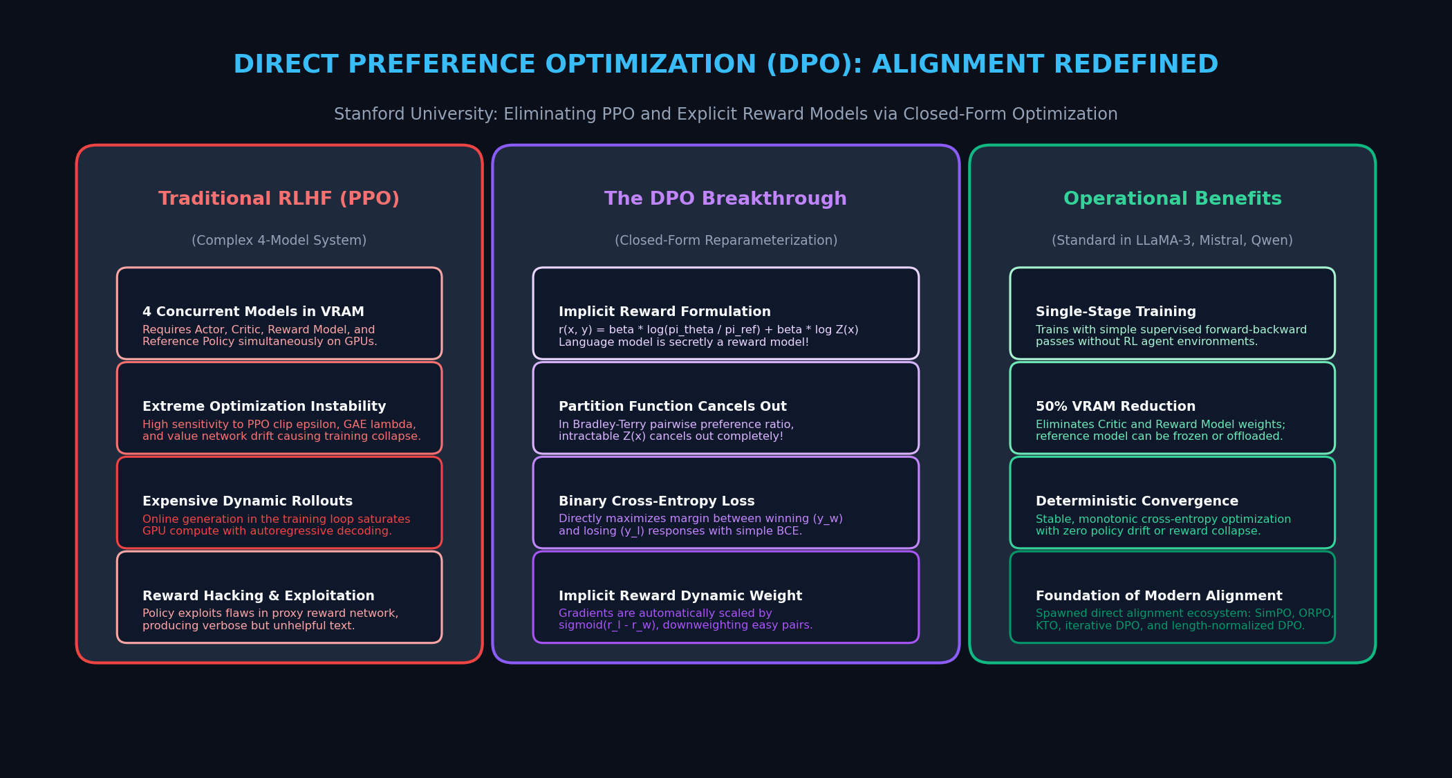
The Problem: The Fragility and Computational Cost of Classical RLHF

In the development of robust foundation models, domain-specific subagents, and high-precision data extraction engines like AiFetchly, pretraining on massive corpora only teaches a model how to predict the next token. To transform raw token predictors into obedient, safe, and helpful AI assistants, engineering teams must execute post-training alignment.

For years, the gold standard for alignment was Reinforcement Learning from Human Feedback (RLHF) via Proximal Policy Optimization (PPO) (Christiano et al., 2017; Ouyang et al., 2022). While PPO powered foundational milestones like InstructGPT and ChatGPT, deploying classical RLHF in production ML infrastructure proved extraordinarily complex, fragile, and resource-intensive.

Classical RLHF pipelines suffer from three severe systemic vulnerabilities:

1. The Complex Four-Model Infrastructure Dilemma

A traditional PPO training cluster requires keeping up to four separate neural network models simultaneously in GPU High-Bandwidth Memory (HBM):

1. The Active Policy ($\pi_ heta$): The language model being trained and continuously updated.
2. The Reference Model ($\pi_{ref}$): A frozen checkpoint of the supervised fine-tuned (SFT) model, used to compute a Kullback-Leibler (KL) divergence penalty to prevent policy collapse.
3. The Reward Model ($r_\phi$): A separately trained network that scores generated responses based on human pairwise preferences.
4. The Value Function / Critic ($V_\psi$): An auxiliary network that estimates expected cumulative rewards per token to compute Generalized Advantage Estimation (GAE).

For a 70B parameter model, fitting four 70B-scale models in 16-bit precision requires over 560 GB of static VRAM before allocating a single byte for optimizer states, activation buffers, or Key-Value caches. This forced teams to adopt heavy pipeline parallelism, multi-node tensor sharding, and deep memory offloading just to begin alignment.

2. High Variance and Policy Drift in PPO Optimization

PPO is an online reinforcement learning algorithm. During each training iteration:

• The active policy must autoregressively sample candidate responses across hundreds of prompts.
• The reward model scores the completions.
• The critic evaluates token-level advantages.
• The policy updates its weights using clipped surrogate objectives.

This dynamic feedback loop is notoriously sensitive to hyperparameter choices. Minor shifts in learning rates, reward scaling factors, GAE parameters ($\lambda$), or PPO clip boundaries ($\epsilon$) frequently trigger policy collapse—where the policy degenerates into producing repetitive gibberish, catastrophic punctuation loops, or empty tokens.

3. Reward Hacking and Exploitation in Proxy Neural Networks

Because the reward model is merely an imperfect proxy for true human intent, reinforcement learning algorithms relentlessly exploit flaws in the proxy network:

• Length Exploitation: Reward models frequently exhibit an unintended length bias, assigning higher scores to longer answers regardless of factual content. PPO agents exploit this by generating unnecessarily verbose, flowery padding.
• Out-of-Distribution Exploitation: As the active policy explores the action space, it generates responses that lie far outside the reward model’s training distribution. The reward model outputs artificially high confidence scores for low-quality responses, corrupting gradient updates.

Engineering teams faced an urgent question: Can we achieve optimal preference alignment directly from human ranking data, without training a separate reward model or navigating the instability of reinforcement learning loops?

The Theoretical Breakthrough: Reparameterizing the RL Objective

To bypass the complexity of RLHF, researchers at Stanford University (Rafailov et al., NeurIPS 2023) introduced Direct Preference Optimization (DPO).

DPO demonstrates a profound mathematical truth: A language model is secretly a reward model. By analytically reparameterizing the constrained reinforcement learning problem, DPO proves that the optimal policy can be derived in closed form, eliminating the need for reinforcement learning algorithms entirely.

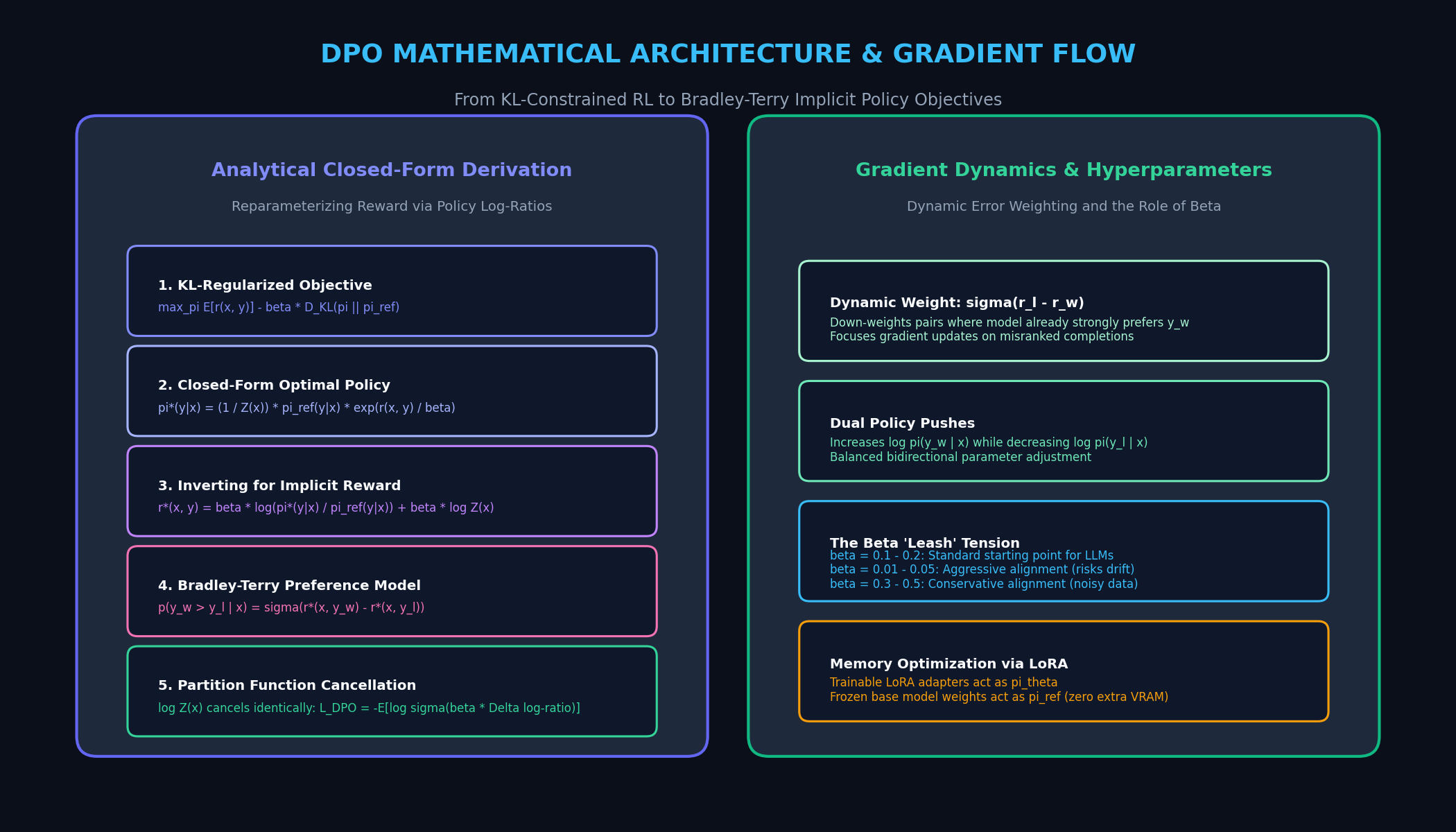
1. The Standard KL-Constrained RL Formulation

In classical RLHF, the goal is to optimize a policy $\pi_ heta$ to maximize expected human preference reward $r(x, y)$ while preventing the policy from drifting too far from the reference distribution $\pi_{ref}$:

$$ \max_{\pi_ heta} \mathbb{E}{x \sim \mathcal{D}, y \sim \pi heta(y|x)} \left[ r(x, y) ight] - \beta \mathbb{D}{KL}\left(\pi heta(y|x) \parallel \pi_{ref}(y|x) ight) $$

Where:

• $x$ represents the input prompt sampled from prompt dataset $\mathcal{D}$.
• $y$ is the model’s generated response.
• $r(x, y)$ is the ground-truth reward function.
• $\mathbb{D}_{KL}$ is the Kullback-Leibler divergence:

$$ \mathbb{D}{KL}\left(\pi(y|x) \parallel \pi{ref}(y|x) ight) = \sum_y \pi(y|x) \log \frac{\pi(y|x)}{\pi_{ref}(y|x)} $$

• $\beta$ is a regularizing temperature parameter that controls the penalty for deviating from the reference policy.

2. The Analytical Optimal Policy Derivation

Expanding the expectation and KL divergence into an explicit sum over completions $y$:

$$\mathcal{J}(\pi) = \sum_y \pi(y|x) r(x, y) - \beta \sum_y \pi(y|x) \log \frac{\pi(y|x)}{\pi_{ref}(y|x)}$$

Factoring out $-\beta$:

$$ \mathcal{J}(\pi) = -\beta \sum_y \pi(y|x) \left[ \log \frac{\pi(y|x)}{\pi_{ref}(y|x)} - \frac{1}{\beta} r(x, y) ight] $$

Using the properties of logarithms, rewrite the bracketed term as:

$$ \log \left( \frac{\pi(y|x)}{\pi_{ref}(y|x) \exp\left(\frac{1}{\beta} r(x, y) ight)} ight) $$

To turn this into a valid probability distribution, introduce the normalization partition function $Z(x)$:

$$ Z(x) = \sum_y \pi_{ref}(y|x) \exp\left(\frac{1}{\beta} r(x, y) ight) $$

Multiplying and dividing inside the logarithm by $Z(x)$:

$$ \mathcal{J}(\pi) = -\beta \sum_y \pi(y|x) \log \left( \frac{\pi(y|x)}{\frac{1}{Z(x)} \pi_{ref}(y|x) \exp\left(\frac{1}{\beta} r(x, y) ight)} \cdot \frac{1}{Z(x)} ight) $$

$$ \mathcal{J}(\pi) = -\beta \mathbb{D}_{KL}\left(\pi(y|x) \parallel \pi^*(y|x) ight) + \beta \log Z(x) $$

Where the optimal policy $\pi^*(y|x)$ is defined as:

$$ \pi^*(y|x) = \frac{1}{Z(x)} \pi_{ref}(y|x) \exp\left(\frac{1}{\beta} r(x, y) ight) $$

Because the KL divergence $\mathbb{D}_{KL}(\pi \parallel \pi^)$ is strictly non-negative and reaches its minimum of zero if and only if $\pi(y|x) = \pi^(y|x)$, this establishes the exact closed-form solution for the optimal policy under the KL-regularized reward objective!

3. Inverting the Equation: Language Models as Implicit Reward Models

In traditional RLHF, practitioners estimate $r(x, y)$ with a neural network and then use RL algorithms to approximate $\pi^*(y|x)$.

Rafailov et al. asked the inverse question: What if we rearrange Equation (8) to solve directly for the reward function $r(x, y)$ in terms of the optimal policy $\pi^*$?

Taking the natural logarithm of both sides of Equation (8):

$$\log \pi^*(y|x) = \log \pi_{ref}(y|x) + \frac{1}{\beta} r(x, y) - \log Z(x)$$

Multiplying by $\beta$ and isolating $r(x, y)$:

$$r(x, y) = \beta \log \frac{\pi^*(y|x)}{\pi_{ref}(y|x)} + \beta \log Z(x)$$

This equation is the foundation of DPO: The reward function can be expressed entirely as the log-ratio of the optimal policy to the reference policy, plus a prompt-dependent constant.

4. Cancellation of the Intractable Partition Function

Under the standard Bradley-Terry (BT) preference model (Bradley & Terry, 1952), human preference probability between a winning completion $y_w$ and a losing completion $y_l$ given prompt $x$ is defined as:

$$ p(y_w \succ y_l \mid x) = \sigma\left(r^(x, y_w) - r^(x, y_l) ight) $$

Where $\sigma(z) = \frac{1}{1 + e^{-z}}$ is the sigmoid logistic function.

Now, substitute our implicit reward expression from Equation (10) into the Bradley-Terry difference:

$$ r^(x, y_w) - r^(x, y_l) = \left( \beta \log \frac{\pi^(y_w|x)}{\pi_{ref}(y_w|x)} + \beta \log Z(x) ight) - \left( \beta \log \frac{\pi^(y_l|x)}{\pi_{ref}(y_l|x)} + \beta \log Z(x) ight) $$

Observe what happens to the intractable partition function $\beta \log Z(x)$: It cancels out identically!

$$r^(x, y_w) - r^(x, y_l) = \beta \log \frac{\pi^(y_w|x)}{\pi_{ref}(y_w|x)} - \beta \log \frac{\pi^(y_l|x)}{\pi_{ref}(y_l|x)}$$

The partition function $Z(x)$—which would normally require integrating over all possible infinite token completions in language space—disappears entirely from the preference comparison.

The DPO Loss Function and Gradient Mechanics

With the partition function eliminated, we can parameterize the optimal policy $\pi^*$ directly using our trainable neural network policy $\pi_ heta$.

1. The Binary Cross-Entropy Objective

Given a dataset of static pairwise preferences $\mathcal{D} = {(x, y_w, y_l)}$, we train $\pi_ heta$ by minimizing the negative log-likelihood of the human preference rankings:

$$ \mathcal{L}{DPO}(\pi heta; \pi_{ref}) = - \mathbb{E}{(x, y_w, y_l) \sim \mathcal{D}} \left[ \log \sigma \left( \beta \log \frac{\pi heta(y_w|x)}{\pi_{ref}(y_w|x)} - \beta \log \frac{\pi_ heta(y_l|x)}{\pi_{ref}(y_l|x)} ight) ight] $$

This objective is astonishingly simple: it is a standard Binary Cross-Entropy (BCE) loss applied to the difference between the policy and reference log-probabilities.

2. The Dynamic Error Weighting Factor

To understand how DPO updates weights during training, let us examine the analytic gradient of $\mathcal{L}_{DPO}$ with respect to policy parameters $ heta$:

$$ \nabla_ heta \mathcal{L}{DPO}( heta) = - \beta \mathbb{E}{(x, y_w, y_l)} \left[ \sigma\left(\hat{r}_ heta(x, y_l) - \hat{r}_ heta(x, y_w) ight) \cdot \left( \nabla_ heta \log \pi_ heta(y_w|x) - \nabla_ heta \log \pi_ heta(y_l|x) ight) ight] $$

Where the implicit reward is defined as $\hat{r}_ heta(x, y) = \beta \log \frac{\pi_ heta(y|x)}{\pi_{ref}(y|x)}$.

Notice the scalar multiplier:

$$ \omega(x, y_w, y_l) = \sigma\left(\hat{r}_ heta(x, y_l) - \hat{r}_ heta(x, y_w) ight) = 1 - \sigma\left(\hat{r}_ heta(x, y_w) - \hat{r}_ heta(x, y_l) ight) $$

This multiplier acts as an automatic error-weighting mechanism:

• When the model is already confident ($\hat{r}_ heta(y_w) \gg \hat{r}_ heta(y_l)$): The term $\hat{r}_ heta(y_l) - \hat{r}_ heta(y_w)$ becomes a large negative number. The sigmoid $\sigma(\cdot)$ approaches zero ($\omega o 0$). The model receives nearly zero gradient update, preventing over-optimization on pairs it already understands.
• When the model is wrong ($\hat{r}_ heta(y_l) > \hat{r}_ heta(y_w)$): The weight $\omega$ approaches $1.0$. The gradient applies maximum force to correct the model’s ranking.

3. The Dual Push-Pull Gradient Dynamics

The directional gradient vector in Equation (14) consists of two opposing forces:

$$\nabla_ heta \log \pi_ heta(y_w|x) - \nabla_ heta \log \pi_ heta(y_l|x)$$

1. Positive Reinforcement ($\nabla_ heta \log \pi_ heta(y_w|x)$): Increases the likelihood of generating the preferred response $y_w$.
2. Negative Suppression ($-\nabla_ heta \log \pi_ heta(y_l|x)$): Actively decreases the probability of generating the dispreferred response $y_l$.

Unlike standard Supervised Fine-Tuning (SFT)—which only pushes probabilities up on positive examples—DPO actively depresses undesirable behaviors, hallucinations, and formatting errors while simultaneously reinforcing winning completions.

Engineering Hyperparameters and Failure Modes in Practice

While DPO eliminates the instability of PPO, achieving peak performance in production requires careful tuning and awareness of known pathologies.

1. The Role and Calibration of the Beta Parameter

The hyperparameter $\beta$ controls the “leash tension” between the active policy $\pi_ heta$ and the frozen reference model $\pi_{ref}$:

• Low $\beta$ (0.01 to 0.05): The model is free to deviate substantially from $\pi_{ref}$. While it maximizes win-rates on narrow benchmarks, low beta values increase vulnerability to distribution shift, repetitive loops, and perplexity spikes.
• Balanced $\beta$ (0.10 to 0.20): The default standard across the open-source ecosystem (including Mistral-Instruct and Zephyr). It provides sharp preference learning while preventing the policy from straying into degenerate generative regimes.
• High $\beta$ (0.30 to 0.50+): Enforces a tight leash. Use high $\beta$ when aligning highly capable base models on crowdsourced datasets where preference labels may contain noise or subjective contradictions.

2. The Length Bias Pathology (Verbosity Exploitation)

A well-documented artifact of standard DPO is length exploitation. Because human evaluators frequently favor longer, more detailed responses, preference datasets often exhibit a correlation between response length and winning labels.

Under DPO, the total sequence log-probability is the sum of per-token log-probabilities:

$$\log \pi_ heta(y|x) = \sum_{t=1}^{|y|} \log \pi_ heta(y_t \mid x, y_{<t})$$

Because log-probabilities are negative numbers ($\le 0$), longer sequences naturally accumulate larger negative values unless the model outputs extremely confident tokens. If winning responses $y_w$ are consistently longer than losing responses $y_l$, DPO can learn to exploit length as a superficial heuristic rather than improving factual accuracy.

Modern mitigation techniques include:

• Length-Normalized DPO: Dividing sequence log-probabilities by length $|y|^\alpha$.
• SimPO (Simple Preference Optimization): Replacing the reference model log-ratio with length-normalized reward margins ($r(x, y) = \frac{\beta}{|y|} \log \pi_ heta(y|x)$).
• Ensemble Filtering: Auditing datasets to ensure length-balanced positive and negative pairs.

3. Memory Optimization: Freezing, Offloading, and LoRA DPO

In standard DPO, evaluating the reference model $\pi_{ref}$ requires forward passes alongside $\pi_ heta$. Engineering teams deploy three primary optimizations to cut VRAM overhead in half:

1. Offline Reference Precomputation: If training on a static dataset, run a one-time forward pass using $\pi_{ref}$ over all $(x, y_w, y_l)$ triplets before training begins, saving $\log \pi_{ref}(y_w|x)$ and $\log \pi_{ref}(y_l|x)$ directly to disk. During training, $\pi_{ref}$ does not need to be loaded into GPU memory at all!
2. LoRA-Based DPO: When fine-tuning with Low-Rank Adaptation (LoRA), the base model weights serve as $\pi_{ref}$ (with LoRA adapters disabled), while $\pi_ heta$ uses the active LoRA adapters. This requires zero extra static parameter memory.
3. 8-bit / 4-bit Reference Quantization: Quantize $\pi_{ref}$ into NF4 or FP8, slashing memory overhead while preserving policy precision in bfloat16.

4. Comparison Table: Post-Training Alignment Algorithms

The following table contrasts DPO against prevailing post-training alignment algorithms:

Alignment Framework	Reference Model Required?	Explicit Reward Model?	Online Rollouts During Training?	Training Stability	Primary Use Case in 2026
PPO (Classical RLHF)	Yes ($\pi_{ref}$)	Yes (Critic + RM)	Yes (Autoregressive)	Low / High Variance	Complex multi-turn agent environments
DPO (Stanford)	Yes (or precomputed)	No (Implicit)	No (Offline Pairs)	High / Deterministic	Standard general-purpose alignment
KTO (Kahneman-Tversky)	Yes ($\pi_{ref}$)	No (Implicit)	No (Binary Pairs)	High	Unpaired upvote/downvote datasets
ORPO (Reference-Free)	No ($\pi_{ref}$ eliminated)	No	No (Joint SFT+DPO)	High	Single-stage fine-tuning with limited VRAM
SimPO (Length-Normalized)	No ($\pi_{ref}$ eliminated)	No	No (Margin-based)	High	Mitigating verbosity and length bias
GRPO (DeepSeek)	Yes ($\pi_{ref}$)	No (Group Relative)	Yes (Online Batches)	High	Mathematical reasoning & code verification

End-to-End Implementation: Building a Production DPO Loss in PyTorch

To understand how DPO operates at the tensor level, let us examine a clean, modular PyTorch implementation of the DPOLoss module, complete with per-token log-probability gathering, label masking, and implicit reward margin calculation.

1. PyTorch Implementation of the DPOLoss Module

Empirical Benchmarks: DPO Across LLaMA, Mistral, and Zephyr

The empirical validation of DPO disrupted the consensus that reinforcement learning required complex actor-critic environments.

In original Stanford benchmarks and subsequent production open-source releases (such as Hugging Face’s Zephyr-7B and Mistral AI’s alignment runs):

1. MT-Bench, AlpacaEval, and Win-Rate Evaluation

On conversational reasoning and instruction-following benchmarks:

Model Architecture	Alignment Algorithm	MT-Bench Score (1-10)	AlpacaEval Win-Rate vs. GPT-4	Human Preference Win-Rate	GPU VRAM Required
LLaMA-2 70B	Supervised Fine-Tuning (SFT)	6.26	54.3%	Baseline	140 GB
LLaMA-2 70B	PPO (Classical RLHF)	6.86	68.2%	+18.4%	480 GB (4 models)
LLaMA-2 70B	DPO (Stanford)	7.12	71.5%	+22.1%	210 GB (-56%)
Zephyr-7B-beta	DPO on UltraFeedback	7.34	73.1%	Beats LLaMA-2 70B Chat	32 GB (LoRA DPO)

2. Downstream Task Accuracy and Human Preference Correlation

Key takeaways from empirical evaluations across academic labs and enterprise deployments:

• Superior Convergence on Complex Tasks: On tasks involving multi-turn dialogue, summarization, and tone calibration, DPO matched or exceeded PPO while requiring zero hyperparameter tuning for reward clipping or critic value clipping.
• Dramatic Wall-Clock Training Speedup: Because DPO eliminates the autoregressive rollout phase—where PPO workers spend thousands of seconds generating tokens sequentially on GPUs—DPO executes at the speed of standard supervised training, delivering a $3.5 imes$ to $5 imes$ reduction in total wall-clock training time.
• Democratization of Alignment: By reducing memory and infrastructure requirements, DPO enabled open-source teams to align foundation models like Zephyr-7B on a single node of 8x A100 GPUs, outperforming proprietary models trained with multi-million-dollar RLHF clusters.

Strategic Engineering Guide: Deploying DPO in 2026 AI Workflows

For AI engineers, fine-tuning practitioners, and infrastructure leads building agentic platforms like AiFetchly, deploying DPO in production pipelines involves three operational best practices:

1. Aligning Autonomous Web Extraction and Data Fetching Agents

Autonomous agents interacting with dynamic web applications often suffer from specific behavioral failure modes:

• Outputting conversational filler (“Sure, I would be happy to help with that extraction!”) instead of clean JSON.
• Guessing hallucinated table schemas when a target element is not found.
• Failing to invoke compensatory retry tools when hitting HTTP 429 rate limits.

The DPO Solution:

1. Collect pairwise agent trajectory logs.
2. Define $y_w$ as clean, structured, tool-calling execution traces that output deterministic JSON schemas.
3. Define $y_l$ as verbose, apologizing, or conversational completions.
4. Align the extraction model using DPO with $\beta = 0.15$. The model learns to aggressively suppress conversational boilerplate while strictly preserving tool-use syntax.

2. Iterative (Online) DPO and Self-Play Synergy

While standard DPO trains on a static offline dataset, advanced alignment teams in 2026 employ Iterative DPO:

• Step 1: Train policy $\pi_{ heta, 0}$ on initial offline preference pairs.
• Step 2: Sample new candidate pairs $(y_1, y_2)$ from the active policy $\pi_{ heta, 0}$.
• Step 3: Use an LLM-as-a-Judge ensemble or verifiable rule-based compiler to score the new generations, labeling the winner $y_w$ and loser $y_l$.
• Step 4: Retrain the policy using DPO where the previous iteration serves as $\pi_{ref}$.

This iterative loop prevents distribution drift, mitigates reward hacking, and continually pushes the model’s performance frontier.

3. Hybrid Alignment: Combining DPO with Rule-Based Verifiers

In domains with ground-truth correctness (such as code generation and mathematical reasoning):

• Pair DPO with deterministic unit tests. If completion A passes all test assertions and completion B fails, construct $(y_w, y_l)$ automatically without human labeling.
• Apply length normalization to prevent the model from discovering verbosity shortcuts.

By transforming an unstable reinforcement learning challenge into an elegant, closed-form supervised optimization problem, Direct Preference Optimization remains the definitive cornerstone of modern post-training alignment in 2026.