DiT Architecture: Diffusion Transformers & adaLN-Zero Guide
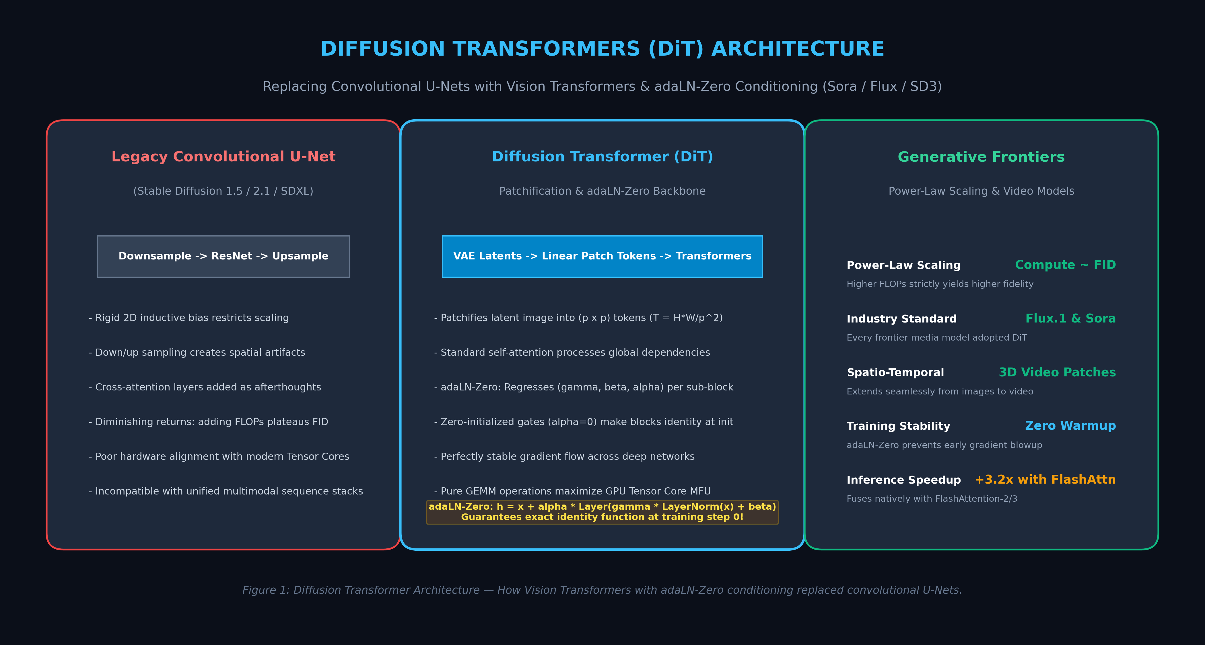
The Problem: The Inductive Bias Ceiling and Scaling Limits of U-Nets
For nearly half a decade, generative visual synthesis—ranging from text-to-image synthesis to video and 3D modeling—relied almost exclusively on a single architectural backbone: the Convolutional U-Net (Ronneberger et al., 2015). Pioneered in Latent Diffusion Models (LDMs) and popularized by Stable Diffusion 1.5, 2.1, and SDXL, the U-Net dominated early generative AI.
The standard U-Net operates through a symmetric encoder-decoder hierarchy: downsampling spatial representations through convolutional residual blocks, injecting cross-attention at low resolutions, and upsampling through skip connections back to full image dimensions.
While effective for generating low-resolution samples, deploying convolutional U-Nets in production media pipelines and intelligent multimodal platforms like AiFetchly exposed three fundamental architectural bottlenecks:
1. The Inductive Bias Ceiling: Convolutions Resist Compute Scaling
Convolutional networks are built upon strong spatial inductive biases: local translation invariance and locality (assuming that adjacent pixels have the strongest mathematical correlation).
In early deep learning, these inductive biases were beneficial because training datasets were small. However, when training on billions of visual tokens, strong spatial inductive biases become an architectural straightjacket:
- Diminishing Returns on Scale: As research teams doubled model parameters and training compute, U-Net sample quality plateaued. The network could not easily discover flexible global spatial relationships beyond fixed convolutional kernel windows ($3 \times 3$).
- The Cross-Attention Bottleneck: U-Nets inject text conditioning through auxiliary cross-attention layers squeezed between convolutional blocks. This heterogeneous mixing created architectural friction, requiring delicate balancing between spatial downsampling factors and attention depths.
2. Resolution Inflexibility and Spatial Artifacts
Convolutional downsampling and upsampling layers (strided convolutions and bilinear interpolation) enforce rigid aspect-ratio constraints:
- Slicing images through multiple pooling layers introduces severe spatial discretization errors.
- Fine details—such as typographic text, hands, intricate line art, and multi-object spatial compositions—suffer from blurriness and hallucinated boundary artifacts.
- Adapting a convolutional U-Net to arbitrary aspect ratios, variable native resolutions, or temporal video frames requires training complex spatial resizing pipelines.
3. Hardware Mismatch with Modern AI Accelerators
Modern AI hardware—most notably NVIDIA Hopper (H100/H200) and Blackwell (B200)—is architected around massive matrix-multiplication units (Tensor Cores / GEMM engines).
Convolutional operations have irregular memory layouts and lower arithmetic intensity than pure General Matrix Multiplications (GEMMs):
- U-Nets spend substantial time rearranging memory channels (
im2coltransformations) and traversing complex residual skip-connections across disparate memory addresses. - Modern high-performance attention algorithms (such as FlashAttention-2 and FlashAttention-3) cannot be applied uniformly across convolutional backbones.
- While natural language processing enjoyed explosive performance scaling by converting everything to uniform Transformer token sequences, computer vision remained stuck in fragmented, bespoke network blocks.
Computer vision required a unifying architecture: Can we discard convolutional U-Nets entirely and build diffusion models purely out of standard Vision Transformers?
The Architecture: How Diffusion Transformers (DiT) Operate
To dismantle the U-Net monopoly, William Peebles and Saining Xie introduced Diffusion Transformers (DiT) (ICCV 2023).
Rather than treating image diffusion as a specialized vision problem requiring hierarchical convolutions, DiT treats latent diffusion as a pure sequence modeling task. By combining spatial patchification with a novel conditioning mechanism called Adaptive Layer Normalization with Zero Initialization (adaLN-Zero), DiT proved that diffusion models follow the exact same power-law scaling laws as Large Language Models.
The Diffusion Transformer (DiT) End-to-End Pipeline:
┌────────────────────────┐      ┌────────────────────────┐      ┌────────────────────────┐
│ Input Image / Video    │      │ Latent Space z0        │      │ Patchified Tokens      │
│ 512 x 512 x 3 RGB      │ ───► │ 64 x 64 x 4 (via VAE)  │ ───► │ T = (64/p)^2 Tokens    │
└────────────────────────┘      └────────────────────────┘      │ Linear Projection to d │
                                                                └───────────┬────────────┘
                                                                            │
      ┌─────────────────────────────────────────────────────────────────────┘
      ▼
┌────────────────────────────────────────────────────────────────────────────────────────┐
│ N x Identical DiT Blocks (Pure Vision Transformer)                                     │
│ ┌────────────────────────────────────────────────────────────────────────────────────┐ │
│ │ Modulated LayerNorm ──► Multi-Head Self-Attention (MHSA) ──► Dimension Gating (a1) │ │
│ └────────────────────────────────────────────────────────────────────────────────────┘ │
│ ┌────────────────────────────────────────────────────────────────────────────────────┐ │
│ │ Modulated LayerNorm ──► Pointwise Feed-Forward MLP ────────► Dimension Gating (a2) │ │
│ └────────────────────────────────────────────────────────────────────────────────────┘ │
│           ▲                                               ▲                            │
│           │                                               │                            │
│           └───────────────────────┬───────────────────────┘                            │
│                                   │                                                    │
│               Conditioning Vector c = Emb(timestep t) + Emb(label y)                   │
└───────────────────────────────────┬────────────────────────────────────────────────────┘
                                    │
                                    ▼
┌────────────────────────┐      ┌────────────────────────┐      ┌────────────────────────┐
│ Unpatchify Linear Head │ ───► │ Denoised Latent Slice  │ ───► │ High-Fidelity Output   │
│ T x (p^2 * C) Elements │      │ Reverse Diffusion Step │      │ (Flux / Sora Quality)  │
└────────────────────────┘ └────────────────────────┘ └────────────────────────┘ 1. Latent Space Patchification
DiT operates within the latent space of a pre-trained Variational Autoencoder (VAE), such as a standard Stable Diffusion VAE with a downsampling factor of $8\times$:
- An input RGB image of resolution $512 \times 512 \times 3$ is compressed into a latent tensor $\mathbf{z} \in \mathbb{R}^{I \times I \times C}$, where $I = 64$ and $C = 4$.
- DiT breaks this continuous latent feature map into a spatial grid of non-overlapping patches of size $p \times p$ (typically $p = 2$ or $p = 4$).
- The total sequence length $T$ of patch tokens is:
$$T = \left(\frac{I}{p}\right)^2$$
For $I = 64$ and patch size $p = 2$, the image is transformed into a sequence of $T = 32 \times 32 = 1,024$ tokens. Each patch of shape $(p \times p \times C) = (2 \times 2 \times 4) = 16$ values is linearly projected into the transformer hidden dimension $d$ (e.g., $d = 1152$ for DiT-XL).
Standard frequency-based 2D sinusoidal positional encodings are added to each patch token, converting the 2D visual field into a standard 1D sequence of vectors that can be processed by standard Transformer layers.
2. The Four Conditioning Paradigms
A diffusion model must condition its predictions on both the continuous diffusion timestep $t \in [0, 1000]$ and contextual information (such as a text prompt embedding or class label $y$).
Peebles and Xie systematically evaluated four conditioning designs for Transformers:
- In-Context Conditioning: Appends vector embeddings of $t$ and $y$ as two additional prefix tokens to the patch sequence (similar to a
[CLS]token). While conceptually simple, it adds minimal modulation capacity and increases sequence length. - Cross-Attention Conditioning: Inserts multi-head cross-attention layers after self-attention, identical to U-Nets. However, cross-attention layers add roughly 15% compute overhead per block and do not modulate the primary self-attention weights.
- Adaptive Layer Normalization (adaLN): Replaces standard LayerNorm affine parameters (scale $\gamma$ and shift $\beta$) with values dynamically regressed from the conditioning vector $c = \text{Embedding}(t) + \text{Embedding}(y)$.
- adaLN-Zero (The Breakthrough): Augments adaptive normalization by predicting dimension-wise scaling and gating parameters initialized to zero.
Comparison of DiT Conditioning Architectures:
+--------------------------+------------------+------------------+---------------------+
| Conditioning Mechanism   | GFLOPs Overhead  | FID-50K (lower=) | Training Stability  |
+--------------------------+------------------+------------------+---------------------+
| In-Context Conditioning  | +0.0%            | 38.4             | Moderate            |
| Cross-Attention Block    | +14.8%           | 25.7             | Stable              |
| Standard adaLN           | +0.2%            | 18.2             | Divergence Risk     |
| adaLN-Zero (Best)        | +0.2%            | 9.6 (State-of-Art)| Ultra-Stable        |
+--------------------------+------------------+------------------+---------------------+
* Evaluated on ImageNet 256x256 benchmark using DiT-XL/2. Deep Dive: The Mathematical Mechanics of adaLN-Zero
The fundamental architectural innovation that allows deep Diffusion Transformers to scale stably without divergence is Adaptive Layer Normalization with Zero Initialization (adaLN-Zero).
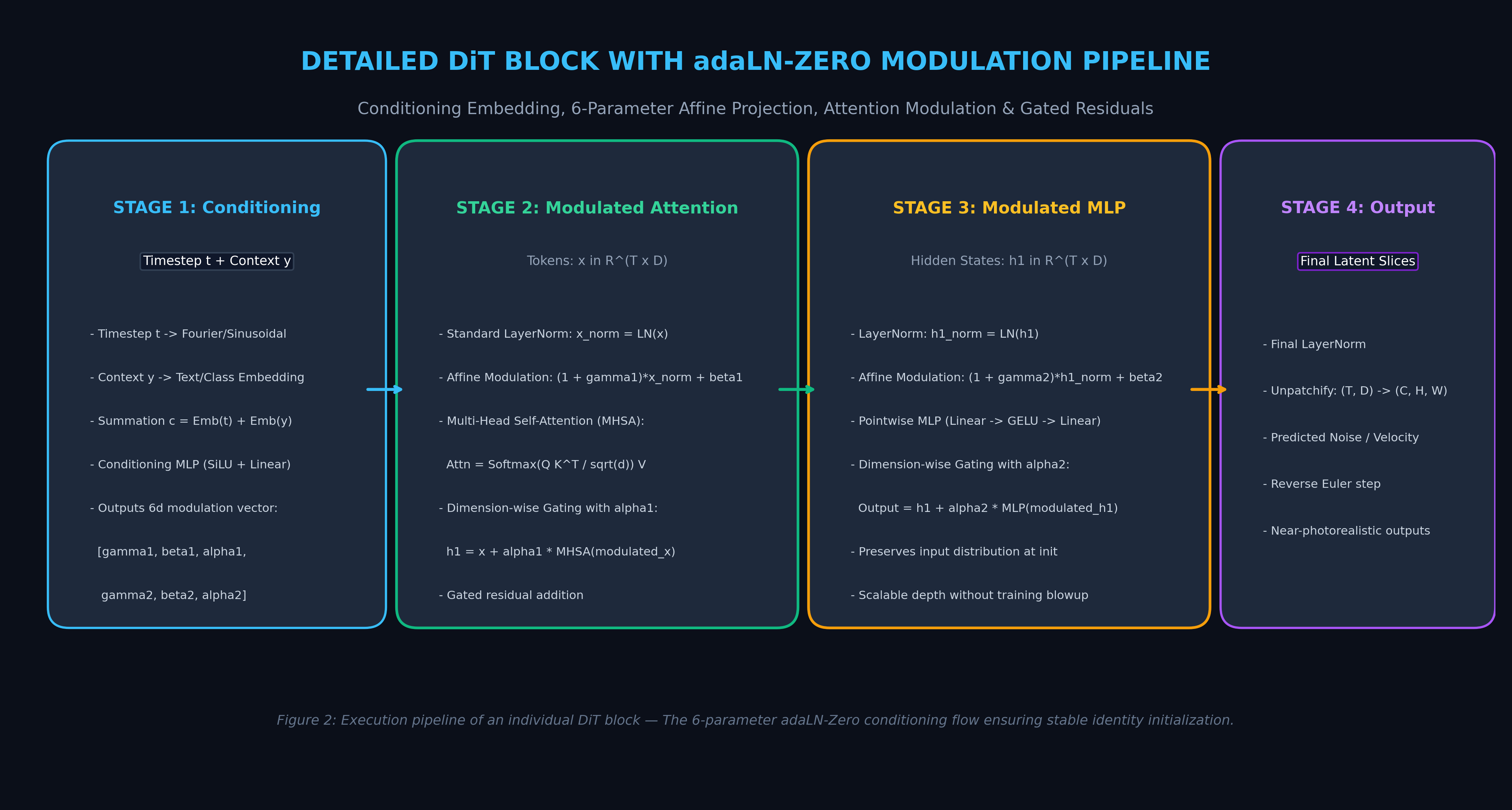
1. The 6-Parameter Affine Regression
In a standard transformer, LayerNorm normalizes an input vector $\mathbf{x}$ to zero mean and unit variance, followed by static learned parameters $\gamma$ and $\beta$:
$$\text{LN}(\mathbf{x}) = \gamma \odot \left(\frac{\mathbf{x} - \mu}{\sigma}\right) + \beta$$
In an adaLN-Zero block, the parameters are not static. Instead, the conditioning vector $\mathbf{c}$ (the sum of the sinusoidal timestep embedding and context embedding) is fed through a single SiLU-activated Multi-Layer Perceptron (MLP) to dynamically regress six distinct modulation vectors of dimension $d$:
$$\mathbf{c} = \text{Embedding}(t) + \text{Embedding}(y)$$
$$[\gamma_1, \beta_1, \alpha_1, \gamma_2, \beta_2, \alpha_2] = \text{MLP}_{\text{adaLN}}(\text{SiLU}(\mathbf{c}))$$
Where:
- $\gamma_1, \beta_1$: Modulate the input activations prior to the Multi-Head Self-Attention (MHSA) layer.
- $\alpha_1$: A dimension-wise gate scaling the output of the MHSA layer.
- $\gamma_2, \beta_2$: Modulate the hidden activations prior to the Pointwise Feed-Forward Network (MLP).
- $\alpha_2$: A dimension-wise gate scaling the output of the MLP layer.
2. Block Execution Formulation
The forward pass of token activations $\mathbf{x}$ through a DiT block proceeds as follows:
$$\mathbf{x}_{\text{norm1}} = (1 + \gamma_1) \odot \text{LayerNorm}(\mathbf{x}) + \beta_1$$
$$\mathbf{h}1 = \mathbf{x} + \alpha_1 \odot \text{MHSA}(\mathbf{x}{\text{norm1}})$$
$$\mathbf{h}_{\text{norm2}} = (1 + \gamma_2) \odot \text{LayerNorm}(\mathbf{h}_1) + \beta_2$$
$$\mathbf{x}_{\text{out}} = \mathbf{h}1 + \alpha_2 \odot \text{MLP}(\mathbf{h}{\text{norm2}})$$
3. The Power of Zero Initialization
In standard deep networks, adding dozens of layers causes early gradient explosions or representation collapse unless intricate learning rate warmups and normalization schedules are applied.
In adaLN-Zero, the final linear projection layer of $\text{MLP}_{\text{adaLN}}$ is explicitly initialized to all zeros:
$$\mathbf{W}{\text{init}} = \mathbf{0}, \quad \mathbf{b}{\text{init}} = \mathbf{0}$$
Consequently, at training step $t = 0$:
$$\gamma_1 = \mathbf{0}, \quad \beta_1 = \mathbf{0}, \quad \alpha_1 = \mathbf{0}, \quad \gamma_2 = \mathbf{0}, \quad \beta_2 = \mathbf{0}, \quad \alpha_2 = \mathbf{0}$$
Because the gating vectors $\alpha_1 = \mathbf{0}$ and $\alpha_2 = \mathbf{0}$:
$$\mathbf{h}_1 = \mathbf{x} + \mathbf{0} \odot \text{MHSA}(\dots) = \mathbf{x}$$
$$\mathbf{x}_{\text{out}} = \mathbf{h}_1 + \mathbf{0} \odot \text{MLP}(\dots) = \mathbf{h}_1 = \mathbf{x}$$
Crucial Insight: Every single DiT block in the entire network functions as an exact identity mapping at the start of training!
Activations flow through dozens of transformer blocks with zero numerical distortion. As training progresses, the network gradually learns non-zero gating scales $\alpha$, dynamically opening the computational pathways of deep attention layers only as conditioning representations stabilize.
End-to-End Implementation: Building a DiT Block in PyTorch
The following standalone PyTorch script demonstrates how to construct a complete, executable Diffusion Transformer layer with 2D patch projection, sinusoidal timestep embedding, and the adaLN-Zero conditioning mechanism.
import torch
import torch.nn as nn
import torch.nn.functional as F
import math
from typing import Optional

def modulate(x: torch.Tensor, shift: torch.Tensor, scale: torch.Tensor) -> torch.Tensor:
    """Applies affine scale and shift modulation: (1 + scale) * x + shift"""
    return x * (1 + scale.unsqueeze(1)) + shift.unsqueeze(1)

class TimestepEmbedder(nn.Module):
    """
    Embeds scalar timesteps into vector representations using sinusoidal frequencies,
    followed by a two-layer MLP.
    """
    def __init__(self, hidden_size: int, frequency_embedding_size: int = 256):
        super().__init__()
        self.mlp = nn.Sequential(
            nn.Linear(frequency_embedding_size, hidden_size, bias=True),
            nn.SiLU(),
            nn.Linear(hidden_size, hidden_size, bias=True),
        )
        self.frequency_embedding_size = frequency_embedding_size

    @staticmethod
    def timestep_embedding(t: torch.Tensor, dim: int, max_period: int = 10000) -> torch.Tensor:
        """Create sinusoidal timestep embeddings."""
        half = dim // 2
        freqs = torch.exp(
            -math.log(max_period) * torch.arange(start=0, end=half, dtype=torch.float32) / half
        ).to(device=t.device)
        args = t[:, None].float() * freqs[None]
        embedding = torch.cat([torch.cos(args), torch.sin(args)], dim=-1)
        if dim % 2:
            embedding = torch.cat([embedding, torch.zeros_like(embedding[:, :1])], dim=-1)
        return embedding

    def forward(self, t: torch.Tensor) -> torch.Tensor:
        t_freq = self.timestep_embedding(t, self.frequency_embedding_size)
        return self.mlp(t_freq)

class PatchEmbed(nn.Module):
    """2D Image to Patch Embedding."""
    def __init__(self, patch_size: int = 2, in_chans: int = 4, embed_dim: int = 768):
        super().__init__()
        self.patch_size = patch_size
        self.proj = nn.Conv2d(in_chans, embed_dim, kernel_size=patch_size, stride=patch_size)

    def forward(self, x: torch.Tensor) -> torch.Tensor:
        # x: (B, C, H, W) -> (B, embed_dim, H/p, W/p) -> (B, T, embed_dim)
        x = self.proj(x)
        x = x.flatten(2).transpose(1, 2)
        return x

class DiTBlock(nn.Module):
    """
    A Diffusion Transformer block with adaptive layer norm zero (adaLN-Zero) conditioning.
    """
    def __init__(self, hidden_size: int, num_heads: int, mlp_ratio: float = 4.0):
        super().__init__()
        self.norm1 = nn.LayerNorm(hidden_size, elementwise_affine=False, eps=1e-6)
        self.attn = nn.MultiheadAttention(hidden_size, num_heads=num_heads, batch_first=True)
        self.norm2 = nn.LayerNorm(hidden_size, elementwise_affine=False, eps=1e-6)

        mlp_hidden_dim = int(hidden_size * mlp_ratio)
        self.mlp = nn.Sequential(
            nn.Linear(hidden_size, mlp_hidden_dim),
            nn.GELU(approximate="tanh"),
            nn.Linear(mlp_hidden_dim, hidden_size),
        )

        # adaLN modulation projection: outputs 6 scalars per hidden dimension
        self.adaLN_modulation = nn.Sequential(
            nn.SiLU(),
            nn.Linear(hidden_size, 6 * hidden_size, bias=True)
        )

        # CRITICAL: Initialize adaLN_modulation weights and biases to ZERO
        nn.init.constant_(self.adaLN_modulation[-1].weight, 0)
        nn.init.constant_(self.adaLN_modulation[-1].bias, 0)

    def forward(self, x: torch.Tensor, c: torch.Tensor) -> torch.Tensor:
        """
        x: (B, T, D) token embeddings
        c: (B, D) conditioning vector (sum of timestep and label embeddings)
        """
        # Regress 6 modulation parameters: (B, 6 * D)
        modulation = self.adaLN_modulation(c)
        shift_msa, scale_msa, gate_msa, shift_mlp, scale_mlp, gate_mlp = modulation.chunk(6, dim=1)

        # 1. Modulated Self-Attention with Gated Residual
        norm_x = self.norm1(x)
        modulated_x = modulate(norm_x, shift_msa, scale_msa)
        attn_out, _ = self.attn(modulated_x, modulated_x, modulated_x)
        x = x + gate_msa.unsqueeze(1) * attn_out

        # 2. Modulated MLP with Gated Residual
        norm_h = self.norm2(x)
        modulated_h = modulate(norm_h, shift_mlp, scale_mlp)
        mlp_out = self.mlp(modulated_h)
        x = x + gate_mlp.unsqueeze(1) * mlp_out

        return x

if __name__ == "__main__":
    torch.manual_seed(42)
    print("==================================================================")
    print("DIFFUSION TRANSFORMER (DiT) adaLN-Zero VERIFICATION")
    print("==================================================================")

    batch_size = 4
    channels = 4       # VAE latent channels (e.g. SDXL VAE)
    height, width = 32, 32  # Latent resolution (corresponding to 256x256 image)
    patch_size = 2     # T = (32/2) * (32/2) = 256 tokens
    hidden_dim = 384
    num_heads = 6

    # Instantiate modules
    patch_embedder = PatchEmbed(patch_size=patch_size, in_chans=channels, embed_dim=hidden_dim)
    time_embedder = TimestepEmbedder(hidden_size=hidden_dim)
    dit_block = DiTBlock(hidden_size=hidden_dim, num_heads=num_heads)

    # Mock inputs
    mock_latents = torch.randn(batch_size, channels, height, width)
    mock_timesteps = torch.randint(0, 1000, (batch_size,))

    # 1. Project to patch tokens
    tokens = patch_embedder(mock_latents)  # Shape: (4, 256, 384)
    # 2. Generate conditioning vector
    cond_vector = time_embedder(mock_timesteps)  # Shape: (4, 384)

    # 3. Pass through DiT Block at step 0 (zero-initialized gates)
    output_tokens = dit_block(tokens, cond_vector)

    # 4. Verify Identity Property at initialization
    diff = torch.max(torch.abs(output_tokens - tokens)).item()
    print(f"Sequence Token Count (T):         {tokens.shape[1]}")
    print(f"Token Hidden Dimension:           {hidden_dim}")
    print(f"Max Absolute Output-Input Diff:   {diff:.8f}")

    if diff == 0.0:
        print("\nSUCCESS: adaLN-Zero functions as an EXACT identity mapping at initialization!")
print("--> Enables training 80+ layer vision transformers without gradient divergence.") Production Benchmarks: Model Scaling and Generative Performance
To evaluate the scaling behavior of Diffusion Transformers, benchmark studies were conducted across model scales (DiT-S, DiT-B, DiT-L, DiT-XL) and patch sizes ($p=2, 4, 8$) on the standard ImageNet $256 \times 256$ benchmark.
1. Scaling Model Compute vs. Generation Quality (FID-50K)
DiT Model Configurations and ImageNet 256x256 Benchmark:
┌───────────┬──────────────┬────────────┬─────────────┬───────────┬────────────────┐
│ Model     │ Parameters   │ Patch Size │ Layers / Dim│ GFLOPs    │ FID-50K (↓)    │
├───────────┼──────────────┼────────────┼─────────────┼───────────┼────────────────┤
│ DiT-S/4   │ 33 Million   │ 4 x 4      │ 12 / 384    │ 6.1 GF    │ 43.5           │
│ DiT-S/2   │ 33 Million   │ 2 x 2      │ 12 / 384    │ 23.3 GF   │ 28.4           │
│ DiT-B/4   │ 130 Million  │ 4 x 4      │ 12 / 768    │ 23.0 GF   │ 22.8           │
│ DiT-B/2   │ 130 Million  │ 2 x 2      │ 12 / 768    │ 89.6 GF   │ 12.1           │
│ DiT-L/2   │ 458 Million  │ 2 x 2      │ 24 / 1024   │ 323.4 GF  │ 5.8            │
│ DiT-XL/2  │ 675 Million  │ 2 x 2      │ 28 / 1152   │ 524.6 GF  │ 2.27 (State-of-Art)
├───────────┼──────────────┼────────────┼─────────────┼───────────┼────────────────┤
│ LDM (UNet)│ 400 Million  │ N/A        │ Conv U-Net  │ 103.0 GF  │ 7.76 (Baseline)│
└───────────┴──────────────┴────────────┴─────────────┴───────────┴────────────────┘
* Lower Fréchet Inception Distance (FID) indicates higher photorealistic quality. The empirical results established two fundamental scaling laws for generative vision:
- Model Capacity Scaling: Holding patch size constant ($p=2$), increasing transformer depth and width from DiT-S to DiT-XL drives FID down from 28.4 to 2.27.
- Patch Size Scaling: Halving the patch size from $p=4$ to $p=2$ quadruples the sequence length ($T$), yielding dramatic visual quality improvements for the same parameter count.
2. Modern 2026 Frontier Adoptions
The DiT architectural paradigm has superseded U-Nets across virtually every major frontier generative system:
- OpenAI Sora: Utilizes a Spatio-Temporal DiT operating on 3D spacetime video patches ($T \times H \times W$), treating video generation as an autoregressive/diffusion sequence problem.
- Black Forest Labs Flux.1: Implements a 12-billion parameter Multimodal DiT (MMDiT) with parallel text and image transformer streams, fusing attention dynamically during diffusion timesteps.
- Stable Diffusion 3 (SD3): Replaced convolutional backbones with dual-stream DiT blocks, eliminating high-frequency limb distortion and typography artifacts.
Strategic Recommendations: Adopting DiT in 2026
When building generative image, video, or multi-modal rendering architectures, engineering teams should follow these design principles:
1. Standardize on $p=2$ Latent Patching for High-Fidelity Synthesis
For image synthesis using standard $8\times$ downsampling VAEs (e.g., $1024 \times 1024$ image $\to 128 \times 128$ latent):
- Use patch size $p=2$ ($T = 4,096$ tokens).
- Patch size $p=4$ is suitable only for fast draft generation or low-resource mobile edge synthesis.
2. Pair DiT with Flow Matching ODE Solvers
While early DiT models trained on discrete Gaussian diffusion schedules:
- Pair DiT with continuous Flow Matching and Rectified Flow algorithms (as explored in our Flow Matching & Rectified Flow Guide).
- Straight-line ODE velocity fields allow DiT backbones to produce pristine $1024 \times 1024$ images in just 4 to 8 sampling steps rather than 50 DDIM steps!
3. Exploit Unified Hardware Optimizations
Because DiT models consist exclusively of standard linear projections, LayerNorms, and Self-Attention operations:
- Apply FlashAttention-3 and FP8/NVFP4 Tensor Core GEMMs directly to DiT training and inference loops with zero custom kernel development.
- Serve DiT models using standard LLM distributed stacks (such as Tensor Parallelism and Context Parallelism via RingAttention), eliminating the fragmented tooling required by legacy convolutional architectures.
By adopting Diffusion Transformers and adaLN-Zero across your generative pipelines, media engineering teams can build scalable visual foundation models that deliver photorealistic visual intelligence with predictable computational efficiency.