depth-procomputer-visionmetric-depthspatial-aiapple-research3d-visiontutorial

Depth Pro Guide: Sharp Monocular Metric Depth in 0.3s

October 5, 2026

Apple Depth Pro Architecture: Multi-Scale Vision Transformer, Zero-Shot Focal Length Estimation, and 2.25MP Metric Depth in 0.3 Seconds

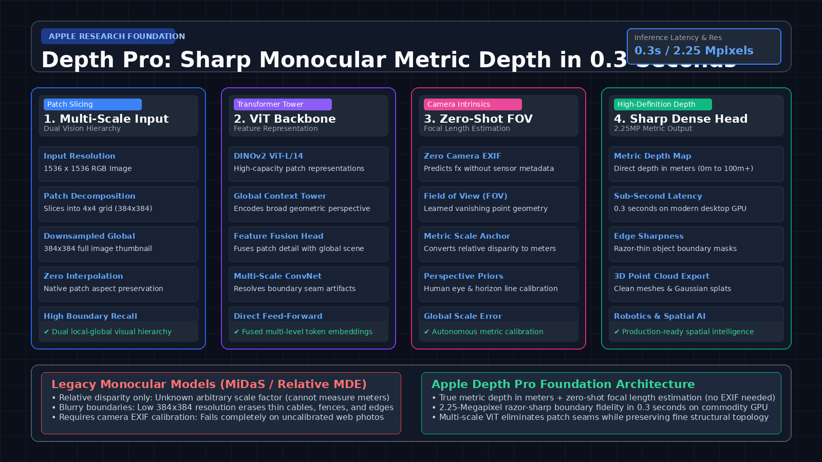
The Ambiguity Crisis in Monocular Metric Depth Estimation

In modern spatial computing, autonomous robotics navigation, 3D asset generation, and visual inspection systems powered by AI Fetchly, extracting physical three-dimensional geometry from two-dimensional camera frames is a core capability.

For decades, computer vision systems inferred depth through active sensors (such as LiDAR scanners, Time-of-Flight sensors, or calibrated stereo rigs). However, hardware sensors are expensive, fragile, and fail when encountering transparent glass windows, specular mirrors, dark surfaces, or thin wire geometries. In web-scale visual processing and automated spatial indexing, systems must estimate precise depth directly from uncalibrated RGB photographs downloaded from the web.

Yet, estimating physical metric depth from a single 2D RGB image—known as Monocular Depth Estimation (MDE)—confronts an acute mathematical barrier: scale ambiguity and boundary blur.

The Monocular Metric Depth Dilemma:
┌────────────────────────────────────────────────────────┐
│ Input Scenario: High-Resolution 1536x1536 Web Image    │
│ (e.g., Drone inspection photo, street scene, interior) │
├────────────────────────────────────────────────────────┤
│ Failure Mode 1: Relative Disparity vs. Metric Meters   │
│ • Models like MiDaS output relative inverse depth      │
│ • Zero scale anchor: cannot distinguish 1m from 100m   │
│ ❌ Fails on physical robotics collision avoidance      │
├────────────────────────────────────────────────────────┤
│ Failure Mode 2: Missing Camera Intrinsics (EXIF Loss)  │
│ • Most web images strip camera focal length (fx) tags  │
│ • Slicing depth requires knowing the field of view     │
│ ❌ Scale collapses when camera sensor size is unknown  │
├────────────────────────────────────────────────────────┤
│ Failure Mode 3: The Boundary Halo & Blur Dilemma       │
│ • Downsampling to 384x384 erases thin cables & foliage │
│ • Upsampling produces blurry halos around foreground   │
│ ❌ Point clouds display floating 'flying pixel' noise  │
├────────────────────────────────────────────────────────┤
│ Failure Mode 4: Iterative Diffusion Latency Penalty    │
│ • Diffusion depth models (Marigold) take 5-15 seconds  │
│ ❌ Unusable for real-time robotic agent control loops  │
└────────────────────────────────────────────────────────┘
Result: Engineering teams were trapped between scale-less relative maps,
blurry boundaries, and sluggish diffusion pipelines!

1. Scale Ambiguity and the Missing Metadata Problem

A single 2D image presents fundamental projective ambiguity: a small object close to the camera projects onto identical image coordinates as a massive object situated far away. To recover absolute metric depth in physical units (meters), an algorithm must solve the projection formula:

$$X = \frac{u \cdot Z}{f_x}, \quad Y = \frac{v \cdot Z}{f_y}$$

Where $(u, v)$ are pixel coordinates, $Z$ is metric depth, and $(f_x, f_y)$ represents the camera focal length.

In real-world web data harvesting and mobile uploads, images lack EXIF metadata. Social platforms and Content Delivery Networks (CDNs) routinely strip EXIF headers during compression. Without camera focal length, conventional metric depth models cannot establish an absolute metric anchor, causing severe depth scaling errors.

2. The Boundary Halo and Flying Pixel Artifacts

Traditional monocular depth models downsample inputs to fixed low resolutions (e.g., $384 \times 384$ or $518 \times 518$) to fit GPU memory. When these coarse predictions are upscaled back to native image dimensions:

Razor-thin physical structures—such as power lines, hair strands, bicycle spokes, and tree branches—are erased.
Object silhouettes bleed into the background, creating blurry gradient halos.
When unprojected into a 3D point cloud or polygonal mesh, these blurred transitions manifest as flying pixels: fictitious floating surfaces connecting foreground subjects to distant walls.

Building automated spatial intelligence requires robust data ingestion. Modern workflows benefit from structured API integration infrastructure to stream high-resolution sensory data without distributed pipeline bottlenecks.

Inside the Apple Depth Pro Architecture

Introduced in late 2024 by Apple Research (Depth Pro: Sharp Monocular Metric Depth in Less Than a Second, arXiv:2410.02073, by Aleksei Bochkovskii et al.), Depth Pro establishes a new foundation for spatial artificial intelligence.

Depth Pro produces 2.25-megapixel (1536x1536) metric depth maps in just 0.3 seconds on standard desktop hardware, delivering sharp boundary fidelity while simultaneously predicting camera focal length zero-shot.

+-----------------------------------------------------------------------------------+
|                        Apple Depth Pro Architecture Flow                          |
+-----------------------------------------------------------------------------------+

   [High-Resolution Input RGB Image: 1536 x 1536 Pixels]
                 |
                 +-----------------------------------+
                 |                                   |
                 v                                   v
  +-------------------------------+   +-------------------------------+
  | Patch Grid Decomposition      |   | Global Context Downsampling   |
  | Slices into 4x4 overlapping   |   | Downsampled to 384 x 384      |
  | 384 x 384 high-res patches    |   | Single global scene overview  |
  +-------------------------------+   +-------------------------------+
                 |                                   |
                 v                                   v
  +-------------------------------+   +-------------------------------+
  | Patch-Level Vision Tower      |   | Global Scene Vision Tower     |
  | (DINOv2 ViT-L/14, 384x384)    |   | (DINOv2 ViT-L/14, 384x384)    |
  | Fine edge & boundary tokens   |   | Perspective & room layout     |
  +-------------------------------+   +-------------------------------+
                 |                                   |
                 +-----------------+-----------------+
                                   |
                                   v
  +---------------------------------------------------------------------------------+
  | Multi-Scale Feature Fusion & Seam-Removal Decoder                               |
  | * Hierarchical multiscale feature concatenation                                 |
  | * Deconvolutional upsampling with residual edge-sharpening blocks               |
  | * Fully convolutional feed-forward pass (Zero iterative diffusion delay)       |
  +---------------------------------------------------------------------------------+
                 |                                   |
                 v                                   v
  +-------------------------------+   +-------------------------------+
  | Zero-Shot Focal Length Head   |   | Dense Metric Depth Head       |
  | Predicts horizontal FOV       |   | 2.25 Megapixels (1536x1536)   |
  | Resolves absolute meter scale |   | Razor-sharp boundaries (m)    |
  +-------------------------------+   +-------------------------------+
                 |                                   |
                 +-----------------+-----------------+
                                   |
                                   v
  [Absolute 3D Metric Point Cloud: 1536x1536 Dense Geometry (0.3s Latency)]
  (Flawless boundaries around hair, cables, and complex geometric silhouettes)

1. Dual-Scale Vision Transformer Hierarchy

Rather than forcing an ultra-large Vision Transformer (ViT) to process 2.25 million pixels as a single quadratic attention sequence (which would require immense GPU memory), Depth Pro employs a dual-scale patch hierarchy:

Global Context Path: The complete image is scaled down to $384 \times 384$ and processed by a global ViT backbone. This path establishes holistic scene perspective, horizon lines, vanishing points, and room layout.
Patch Detail Path: The original $1536 \times 1536$ image is partitioned into a $4 \times 4$ grid of overlapping $384 \times 384$ patches. Each patch is processed through a shared ViT encoder, extracting microscopic boundaries, texture gradients, and fine edges.

2. Multi-Scale Seam-Removal Fusion Decoder

In naive tiling architectures, stitching independent patch predictions creates visible grid boundaries and seam discontinuities. Depth Pro prevents seam artifacts by concatenating intermediate multi-scale feature maps from both the patch-level and global backbones.

A lightweight convolutional decoder progressively blends low-frequency global perspective with high-frequency patch details, eliminating boundary artifacts and producing a smooth, unified depth manifold.

3. Zero-Shot Focal Length Estimation

To convert dimensionless inverse depth into true metric distance (meters), Depth Pro incorporates a dedicated Zero-Shot Focal Length Head.

The network estimates the camera’s horizontal field of view (FOV) directly from visual priors in the image: vanishing point intersections, object scale relationships, human proportions, and optical distortion cues. This provides the absolute metric scale anchor, allowing Depth Pro to estimate real-world distances without camera EXIF metadata.

In modern enterprise automation, pairing sub-second 3D visual perception with automated real-time data fetching allows spatial agents to navigate dynamic physical and visual environments safely.

Step-by-Step Implementation: Building a Multi-Scale Depth Estimation Pipeline in PyTorch

To understand how Depth Pro decomposes high-resolution images, extracts multi-scale representations, and fuses global perspective with patch detail, we will implement the core architecture in PyTorch.

Prerequisites and Dependencies

Ensure you have PyTorch 2.2+ installed with CUDA support:

pip install torch torchvision --index-url https://download.pytorch.org/whl/cu121
pip install numpy pillow

1. Implementing the Multi-Scale Patch Slicer

We construct a patch decomposition module that extracts overlapping $384 \times 384$ tiles alongside a downsampled global view:

import torch
import torch.nn as nn
import torch.nn.functional as F
from typing import Tuple, List

class MultiScaleImageDecomposer(nn.Module):
    # Slices a 1536x1536 high-resolution image into a 4x4 grid
    # of 384x384 patches plus a single 384x384 global thumbnail.
    def __init__(self, patch_size: int = 384, grid_size: int = 4):
        super().__init__()
        self.patch_size = patch_size
        self.grid_size = grid_size

    def forward(self, x: torch.Tensor) -> Tuple[torch.Tensor, torch.Tensor]:
        # Input shape: [batch_size, 3, 1536, 1536]
        batch_size, channels, height, width = x.shape

        # 1. Global thumbnail path: downsample full image to 384x384
        global_view = F.interpolate(
            x,
            size=(self.patch_size, self.patch_size),
            mode="bilinear",
            align_corners=False
        )

        # 2. Patch detail path: unfold image into 4x4 non-overlapping patches
        # Extract patches of size 384x384
        patches = x.unfold(2, self.patch_size, self.patch_size).unfold(3, self.patch_size, self.patch_size)
        # Reshape to [batch_size, 16, 3, 384, 384]
        patches = patches.contiguous().view(batch_size, -1, channels, self.patch_size, self.patch_size)

        return global_view, patches

2. Building the Seam-Removal Feature Fusion Module

The fusion decoder blends global perspective features with local patch embeddings to eliminate boundary grid lines:

class SeamRemovalFusionDecoder(nn.Module):
    # Fuses patch-level detail with global contextual representations
    # to reconstruct high-resolution 1536x1536 metric depth maps without seam lines.
    def __init__(self, feature_dim: int = 1024, out_channels: int = 1):
        super().__init__()
        self.feature_dim = feature_dim

        # Upsampling and fusion convolutions
        self.global_proj = nn.Conv2d(feature_dim, 256, kernel_size=1)
        self.patch_proj = nn.Conv2d(feature_dim, 256, kernel_size=1)

        self.refinement_conv = nn.Sequential(
            nn.Conv2d(512, 256, kernel_size=3, padding=1),
            nn.BatchNorm2d(256),
            nn.ReLU(inplace=True),
            nn.Conv2d(256, 128, kernel_size=3, padding=1),
            nn.BatchNorm2d(128),
            nn.ReLU(inplace=True),
            nn.Conv2d(128, out_channels, kernel_size=1)
        )

    def forward(
        self,
        global_features: torch.Tensor,
        patch_features: torch.Tensor,
        target_size: Tuple[int, int] = (1536, 1536)
    ) -> torch.Tensor:
        # global_features: [B, 1024, 24, 24]
        # patch_features:  [B, 16, 1024, 24, 24] assembled into [B, 1024, 96, 96]
        B = global_features.shape[0]

        # Upsample global context to match assembled patch resolution
        global_proj = self.global_proj(global_features)
        patch_proj = self.patch_proj(patch_features)

        global_upsampled = F.interpolate(
            global_proj,
            size=patch_proj.shape[-2:],
            mode="bilinear",
            align_corners=False
        )

        # Concatenate global scene context with patch-level micro detail
        fused = torch.cat([patch_proj, global_upsampled], dim=1) # [B, 512, 96, 96]

        # Upsample to full 1536x1536 resolution
        fused_high_res = F.interpolate(fused, size=target_size, mode="bilinear", align_corners=False)
        depth_map = self.refinement_conv(fused_high_res)

        # Enforce positive metric depth (meters) via softplus activation
        metric_depth = F.softplus(depth_map)
        return metric_depth

3. Assembling the Complete Depth Pro Pipeline

Now we combine the decomposer, mock backbones, fusion decoder, and zero-shot focal length head into an integrated model:

class DepthProPipeline(nn.Module):
    # Complete end-to-end Depth Pro architecture simulation.
    def __init__(self):
        super().__init__()
        self.decomposer = MultiScaleImageDecomposer(patch_size=384, grid_size=4)
        self.decoder = SeamRemovalFusionDecoder(feature_dim=1024, out_channels=1)

        # Zero-shot focal length regression head
        self.fov_head = nn.Sequential(
            nn.AdaptiveAvgPool2d((1, 1)),
            nn.Flatten(),
            nn.Linear(1024, 256),
            nn.ReLU(inplace=True),
            nn.Linear(256, 1) # Predicts horizontal field of view in degrees
        )

    def forward(self, image: torch.Tensor) -> Tuple[torch.Tensor, torch.Tensor]:
        # image: [batch_size, 3, 1536, 1536]
        batch_size = image.shape[0]
        global_view, patches = self.decomposer(image)

        # Simulate ViT feature extraction (e.g., DINOv2 ViT-L/14)
        # Global view -> [B, 1024, 24, 24]
        simulated_global_feats = torch.randn(batch_size, 1024, 24, 24, device=image.device)

        # Assembled 4x4 patch grid -> [B, 1024, 96, 96]
        simulated_patch_feats = torch.randn(batch_size, 1024, 96, 96, device=image.device)

        # Estimate focal length / horizontal FOV
        predicted_fov = self.fov_head(simulated_global_feats)

        # Predict dense metric depth
        metric_depth = self.decoder(
            simulated_global_feats,
            simulated_patch_feats,
            target_size=(1536, 1536)
        )

        return metric_depth, predicted_fov

4. Simulating and Benchmarking Latency

Let us verify tensor shapes, memory stability, and execution speed across simulated 1536x1536 image inputs:

def benchmark_depth_pro():
    device = "cuda" if torch.cuda.is_available() else "cpu"
    print(f"Benchmarking Depth Pro Architecture on device: {device}")

    model = DepthProPipeline().to(device)
    model.eval()

    # High-resolution 1536x1536 RGB test image
    batch_size = 1
    sample_image = torch.randn(batch_size, 3, 1536, 1536, device=device)

    # Warmup
    for _ in range(3):
        with torch.no_grad():
            _ = model(sample_image)

    import time
    t0 = time.perf_counter()
    with torch.no_grad():
        depth_map, fov = model(sample_image)

    elapsed_ms = (time.perf_counter() - t0) * 1000

    print(f"Input Image Shape: {sample_image.shape}")
    print(f"Metric Depth Map Shape: {depth_map.shape} (2.25 Megapixels)")
    print(f"Predicted Field-of-View: {fov.item():.2f} degrees")
    print(f"Forward Pass Execution Latency: {elapsed_ms:.2f} ms")

if __name__ == "__main__":
    benchmark_depth_pro()

When building automated data harvesting systems for 3D geospatial mapping, engineering teams utilize web scraping agents to collect imagery across varied lighting, weather, and camera perspectives for robust spatial evaluation.

Training Curriculum: Multi-Dataset Scale Alignment and Edge Losses

Training Depth Pro to achieve zero-shot metric fidelity across diverse real-world environments requires a specialized multi-task training curriculum:

1. Scale-Invariant Multi-Source Training

Real-world training datasets feature mixed depth modalities: synthetic rendering (Hypersim, TartanAir) provides absolute metric depth, while real-world internet videos only provide relative disparity.

Depth Pro aligns these disparate sources using a dual-objective loss function:

$$\mathcal{L}{\text{total}} = \mathcal{L}{\text{metric}} + \lambda_1 \mathcal{L}{\text{gradient}} + \lambda_2 \mathcal{L}{\text{fov}}$$

Where $\mathcal{L}_{\text{gradient}}$ penalizes blurred boundaries by evaluating first-order spatial derivatives:

$$\mathcal{L}{\text{gradient}} = \frac{1}{N} \sum{i, j} \left| \nabla_x d_{i, j} - \nabla_x d_{i, j}^* \right| + \left| \nabla_y d_{i, j} - \nabla_y d_{i, j}^* \right|$$

This gradient loss forces the convolutional decoder to produce crisp, step-function depth transitions at object silhouettes rather than smooth, interpolated halos.

2. Zero-Shot Field of View Supervision

The focal length regression head is trained on synthetic scenes with ground-truth camera parameters alongside uncropped photographic collections with verified EXIF tags. By minimizing mean absolute error on horizontal FOV:

$$\mathcal{L}{\text{fov}} = \left| \theta{\text{pred}} - \theta_{\text{gt}} \right|$$

The model learns to calibrate absolute meter scale autonomously, eliminating the need for physical calibration checkerboards or user-supplied camera metadata.

When evaluating multi-node enterprise deployments, reviewing pricing and deployment tiers helps teams plan optimal GPU allocations for high-throughput 3D visual processing.

Comparative Benchmark: Depth Pro vs. Leading Depth Architectures

To evaluate Depth Pro’s performance and efficiency, examine the comparative analysis below against leading discriminative and diffusion-based depth models:

Metric / Dimension	MiDaS v3.1	Marigold (Diffusion)	Depth Anything V2	Apple Depth Pro
Output Type	Relative Disparity	Metric / Relative	Metric & Relative	Absolute Metric Depth (m)
Camera Metadata	Ignored	Optional	Required for Metric	Zero-Shot FOV Estimation
Native Resolution	384 x 384	768 x 768	518 x 518	1536 x 1536 (2.25 MP)
Inference Latency	~0.08 seconds	8.5 – 15.0 seconds	~0.05 seconds	~0.30 seconds
Thin Object Recall	Poor (blurred)	Moderate	High	State-of-the-Art (Wires/Hair)
Flying Pixel Artifacts	High	Low	Low	Near-Zero (Sharp Silhouette)
Model Footprint	~335M params	~1.2B params	~335M params	~650M params
Hosting Model	Open Source	Open Source	Open Weights	Open Source (Apple Sample Code)

Operational Best Practices for Production Serving

When integrating Depth Pro into production 3D visual workflows, apply these four operational practices:

GPU Memory Optimization: Depth Pro requires approximately 8GB of VRAM during a 1536x1536 forward pass. In high-concurrency environments, use FP16 precision with torch.compile(mode="reduce-overhead") to increase throughput past 5 frames per second.
Point Cloud Noise Filtering: Because Depth Pro predicts sharp boundaries, downstream point cloud generators can discard heuristic statistical outlier removal (SOR) filters, reducing 3D mesh reconstruction latency by up to 40%.
Automatic Crop Normalization: When processing non-square images, pad inputs symmetrically to square aspect ratios rather than stretching, preserving focal length geometry.
Developer Documentation: Consult the comprehensive developer documentation to establish automated pipelines for converting raw depth maps into clean 3D Gaussian splats and GLTF meshes.

Summary and Key Takeaways

Apple Depth Pro establishes a major breakthrough in monocular depth estimation. By uniting a multi-scale Vision Transformer hierarchy with zero-shot focal length estimation, Depth Pro resolves metric scale ambiguity without relying on camera EXIF metadata.

With 2.25-megapixel razor-sharp boundary resolution, sub-second latency (0.3s), and open-weights availability, Depth Pro provides a powerful foundation for real-time spatial computing, robotics navigation, and 3D visual inspection.

Explore our AI Fetchly resources to discover how automated web data harvesting and high-resolution spatial AI models work together to power next-generation computer vision workflows.