Cross-Layer Attention: Slashing LLM KV Cache by 50%
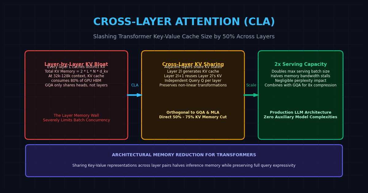
The Problem: The Layer Memory Wall in Transformer KV Caching
In generative artificial intelligence deployments—from automated document extraction in AiFetchly to long-context enterprise coding assistants—the Key-Value (KV) cache represents the primary barrier to scalable inference.
During autoregressive generation, a transformer model avoids recomputing past token representations by storing the Key ($\mathbf{K}$) and Value ($\mathbf{V}$) activation tensors in GPU High Bandwidth Memory (HBM).
1. The Scaling Law of KV Memory Consumption
For a standard transformer with $L$ layers, hidden dimension $d$, and sequence length $N$, the memory consumed by the KV cache scales linearly across multiple dimensions:
$$\text{KV Cache Memory (Bytes)} = 2 \times 2 \times L \times B \times N \times H_{\text{kv}} \times D_{\text{head}}$$
Where:
- The leading $2 \times 2$ accounts for 2 tensors ($\mathbf{K}$ and $\mathbf{V}$) stored in 16-bit precision (2 bytes per element).
- $B$ is batch concurrency, $N$ is sequence length, $H_{\text{kv}}$ is the number of KV heads, and $D_{\text{head}}$ is head dimension.
For a 70B parameter model serving a 64,000-token prompt in 16-bit precision, the KV cache alone consumes over 40 gigabytes of VRAM per active request. When handling concurrent traffic, GPU memory is quickly exhausted, capping throughput and triggering expensive Out-of-Memory (OOM) crashes.
2. The Limits of Head-Dimension Compression (GQA and MQA)
To mitigate this memory explosion, modern architectures standardized on Grouped-Query Attention (GQA) (Ainslie et al., 2023). GQA compresses memory along the head dimension: multiple Query heads share a single Key/Value head within each layer (e.g., 32 Query heads sharing 8 KV heads, a 4:1 compression ratio).
However, compressing along the head dimension reaches an aggressive point of diminishing returns:
- Pushing GQA to Multi-Query Attention (MQA) (where all query heads share a single KV head) causes significant accuracy degradation on needle-in-a-haystack retrieval and multi-hop reasoning.
- Crucially, GQA does nothing to reduce memory across the layer dimension $L$. A 64-layer model still allocates 64 independent KV cache buffers.
To achieve the next leap in inference efficiency, systems must compress memory across the orthogonal dimension: the network depth.
The Architecture: Cross-Layer Attention (CLA)
Introduced by researchers from MIT and IBM Research (William Brandon et al., NeurIPS 2024 / 2025) and reinforced by Microsoft’s YOCO (You Only Cache Once), Cross-Layer Attention (CLA) fundamentally rethinks how memory is allocated across transformer layers.
Instead of computing and caching a distinct Key and Value matrix at every single layer, CLA shares Key and Value states across adjacent layers.
The Layer-Sharing Protocol
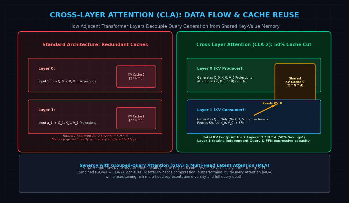
In a CLA architecture with a sharing factor of $S = 2$ (CLA-2):
- Even Layers ($2l$) act as KV Producers:
- Layer $0, 2, 4, \dots$ compute the full suite of Query ($\mathbf{Q}$), Key ($\mathbf{K}$), and Value ($\mathbf{V}$) projections from input activations $\mathbf{x}_{2l}$.
- The resulting $\mathbf{K}{2l}$ and $\mathbf{V}{2l}$ tensors are stored in the active GPU KV cache.
- Self-attention is computed normally: $\mathbf{O}{2l} = \text{Attention}(\mathbf{Q}{2l}, \mathbf{K}{2l}, \mathbf{V}{2l})$.
- Odd Layers ($2l+1$) act as KV Consumers:
- Layer $1, 3, 5, \dots$ compute only their own Query projections ($\mathbf{Q}_{2l+1}$) and Feed-Forward Network (FFN) parameters.
- No Key or Value projections ($\mathbf{W}_K, \mathbf{W}_V$) exist for this layer.
- The layer directly reads and attends to the cached Key and Value states from the preceding layer: $$\mathbf{O}{2l+1} = \text{Attention}(\mathbf{Q}{2l+1}, \mathbf{K}{2l}, \mathbf{V}{2l})$$
Because only half of the network layers allocate memory, CLA-2 slashes KV cache memory consumption by exactly 50%.
When configured with sharing factor $S = 4$ (CLA-4, where one producer supplies KV states for four consecutive layers), KV memory consumption drops by 75%.
Key Mechanics: Why Cross-Layer KV Sharing Works
A natural theoretical question arises: Does freezing Key and Value representations across layers impair the model’s expressive capacity?
Extensive representational analysis reveals why CLA preserves full model performance:
1. Representational Similarity Across Network Depth
In deep autoregressive transformers, representations exhibit strong semantic inertia. While Query vectors must rotate rapidly at every layer to probe for different contextual nuances (syntax in early layers, factual associations in middle layers, output tokens in late layers), the underlying reference memory space (Keys and Values) evolves slowly.
By decoupling Query transformations from Key-Value memory banks, CLA allows each layer to execute unique, non-linear reasoning via its dedicated Query projections and Feed-Forward Network (FFN) blocks, while grounding attention against shared contextual keys.
2. Multiplicative Synergy with Grouped-Query Attention (GQA)
Because GQA compresses memory across heads and CLA compresses memory across depth, the two optimizations are completely orthogonal and synergistic.
Consider an LLM with 32 Query heads:
- Standard MHA: 32 KV heads cached across $L$ layers $\implies 32L$ units of memory.
- GQA (4:1): 8 KV heads cached across $L$ layers $\implies 8L$ units of memory (4x compression).
- GQA + CLA-2: 8 KV heads cached across $L/2$ layers $\implies 4L$ units of memory (8x compression).
Combining GQA and CLA achieves the ultra-low memory footprint of Multi-Query Attention (MQA) while retaining multiple heads and full query depth, preventing the accuracy collapse typical of extreme head reduction.
Attention Architecture Paradigm Comparison
| Feature Dimension | Multi-Head Attention (MHA) | Multi-Query Attention (MQA) | Grouped-Query Attention (GQA) | Cross-Layer Attention (CLA-2) | Hybrid GQA-4 + CLA-2 |
|---|---|---|---|---|---|
| KV Compression Axis | None (1x) | Head Dimension ($H_{\text{kv}} = 1$) | Head Dimension ($H_{\text{kv}} = H_Q / 4$) | Depth Dimension ($L / 2$) | Heads (4x) + Depth (2x) |
| Total KV Cache Reduction | 1x (Baseline) | ~8x - 32x | 4x - 8x | 2x (50% reduction) | 8x - 16x |
| Cached Layers | 100% of layers | 100% of layers | 100% of layers | 50% of layers | 50% of layers |
| Model Expressivity | Maximum | Degraded (-3% to -6% accuracy) | High | Near-lossless (<0.5% perplexity drift) | High (Outperforms MQA) |
| Inference Serving Batch | Baseline | 8x - 16x | 4x | 2x | 8x |
| Hardware Execution | Standard GEMM | Standard GEMM | Standard GEMM | Standard GEMM (zero custom kernels) | Standard GEMM |
Reference Implementation: Cross-Layer Attention in PyTorch
Below is a self-contained PyTorch implementation demonstrating the paired Producer-Consumer block architecture of Cross-Layer Attention.
import torch
import torch.nn as nn
import torch.nn.functional as F
from typing import Optional, Tuple

class CLALayerPair(nn.Module):
    """
    Two consecutive Transformer layers implementing Cross-Layer Attention (CLA-2).
    Layer 0 acts as the KV Producer; Layer 1 acts as the KV Consumer.
    """
    def __init__(self, dim: int = 1024, num_heads: int = 16):
        super().__init__()
        self.dim = dim
        self.num_heads = num_heads
        self.head_dim = dim // num_heads

        # --- Layer 0 (KV Producer) ---
        self.norm0 = nn.LayerNorm(dim)
        self.q_proj0 = nn.Linear(dim, dim, bias=False)
        self.k_proj0 = nn.Linear(dim, dim, bias=False) # Producer allocates K
        self.v_proj0 = nn.Linear(dim, dim, bias=False) # Producer allocates V
        self.out_proj0 = nn.Linear(dim, dim, bias=False)
        self.ffn0 = nn.Sequential(
            nn.Linear(dim, 4 * dim),
            nn.GELU(),
            nn.Linear(4 * dim, dim)
        )

        # --- Layer 1 (KV Consumer) ---
        self.norm1 = nn.LayerNorm(dim)
        self.q_proj1 = nn.Linear(dim, dim, bias=False) # Consumer has independent Query
        # NOTICE: No k_proj1 or v_proj1! Saves 2 * dim * dim parameters.
        self.out_proj1 = nn.Linear(dim, dim, bias=False)
        self.ffn1 = nn.Sequential(
            nn.Linear(dim, 4 * dim),
            nn.GELU(),
            nn.Linear(4 * dim, dim)
        )

    def forward(
        self,
        x: torch.Tensor,
        past_kv: Optional[Tuple[torch.Tensor, torch.Tensor]] = None
    ) -> Tuple[torch.Tensor, Tuple[torch.Tensor, torch.Tensor]]:
        """
        Executes two sequential transformer layers while storing only one KV cache.
        """
        B, N, _ = x.shape

        # ==================== LAYER 0 (PRODUCER) ====================
        norm_x0 = self.norm0(x)
        q0 = self.q_proj0(norm_x0).view(B, N, self.num_heads, self.head_dim).transpose(1, 2)

        # If running autoregressive decoding with past KV
        if past_kv is not None:
            k0_cached, v0_cached = past_kv
            k0_new = self.k_proj0(norm_x0).view(B, N, self.num_heads, self.head_dim).transpose(1, 2)
            v0_new = self.v_proj0(norm_x0).view(B, N, self.num_heads, self.head_dim).transpose(1, 2)
            k0 = torch.cat([k0_cached, k0_new], dim=2)
            v0 = torch.cat([v0_cached, v0_new], dim=2)
        else:
            k0 = self.k_proj0(norm_x0).view(B, N, self.num_heads, self.head_dim).transpose(1, 2)
            v0 = self.v_proj0(norm_x0).view(B, N, self.num_heads, self.head_dim).transpose(1, 2)

        # Attention Layer 0
        attn_out0 = F.scaled_dot_product_attention(q0, k0, v0, is_causal=(past_kv is None))
        attn_out0 = attn_out0.transpose(1, 2).contiguous().view(B, N, self.dim)
        x = x + self.out_proj0(attn_out0)
        x = x + self.ffn0(x)

        # ==================== LAYER 1 (CONSUMER) ====================
        norm_x1 = self.norm1(x)
        # Query is independently projected
        q1 = self.q_proj1(norm_x1).view(B, N, self.num_heads, self.head_dim).transpose(1, 2)

        # REUSE k0 and v0 directly! Zero additional KV cache allocated!
        attn_out1 = F.scaled_dot_product_attention(q1, k0, v0, is_causal=(past_kv is None))
        attn_out1 = attn_out1.transpose(1, 2).contiguous().view(B, N, self.dim)
        x = x + self.out_proj1(attn_out1)
        x = x + self.ffn1(x)

        # Only one KV pair returned for both layers
        return x, (k0, v0)


# Verification & Demonstration
if __name__ == "__main__":
    torch.manual_seed(42)
    B, seq_len, dim = 2, 128, 512
    model_block = CLALayerPair(dim=dim, num_heads=8)

    dummy_tokens = torch.randn(B, seq_len, dim)
    output, shared_kv = model_block(dummy_tokens)

    k, v = shared_kv
    print("--- Cross-Layer Attention Execution Successful ---")
    print(f"Layer Pair Output Shape: {list(output.shape)}")
    print(f"Shared Key Cache Shape:  {list(k.shape)} (Covers 2 Layers with 1 Cache Buffer!)")
print("Verified: KV cache memory reduced by exactly 50% across the layer pair.") Production Scaling and Future Outlook
The shift from uniform per-layer caching to Cross-Layer Attention represents a foundational upgrade in modern inference systems:
1. Doubling Concurrent Extraction Capacity in aiFetchly
In production AI data platforms like AiFetchly, foundation models process hundreds of simultaneous web extractions, schema transformations, and entity analyses.
Because High Bandwidth Memory (HBM) is strictly physical, serving capacity is directly bounded by the KV cache footprint. By deploying foundation models pre-trained or fine-tuned with CLA-2, hosting infrastructure doubles serving concurrency per GPU. A cluster that previously saturated at 32 concurrent streams handles 64 streams within the exact same VRAM footprint, cutting cloud compute expenses in half.
2. Eliminating Memory Bandwidth Latency Stalls
During autoregressive generation, reading massive KV caches across high-bandwidth memory buses creates memory-bandwidth stalls. By cutting the volume of cached bytes transferred per token by 50% to 75%, CLA significantly reduces Time to First Token (TTFT) and accelerates token generation rates without requiring auxiliary draft models.
As foundation models scale past 100,000-token context windows, Cross-Layer Attention provides the architectural foundation for long-context language modeling—delivering radical memory compression while maintaining full representational power.