CoTracker3 Guide: Dense Point Tracking in Video with AI
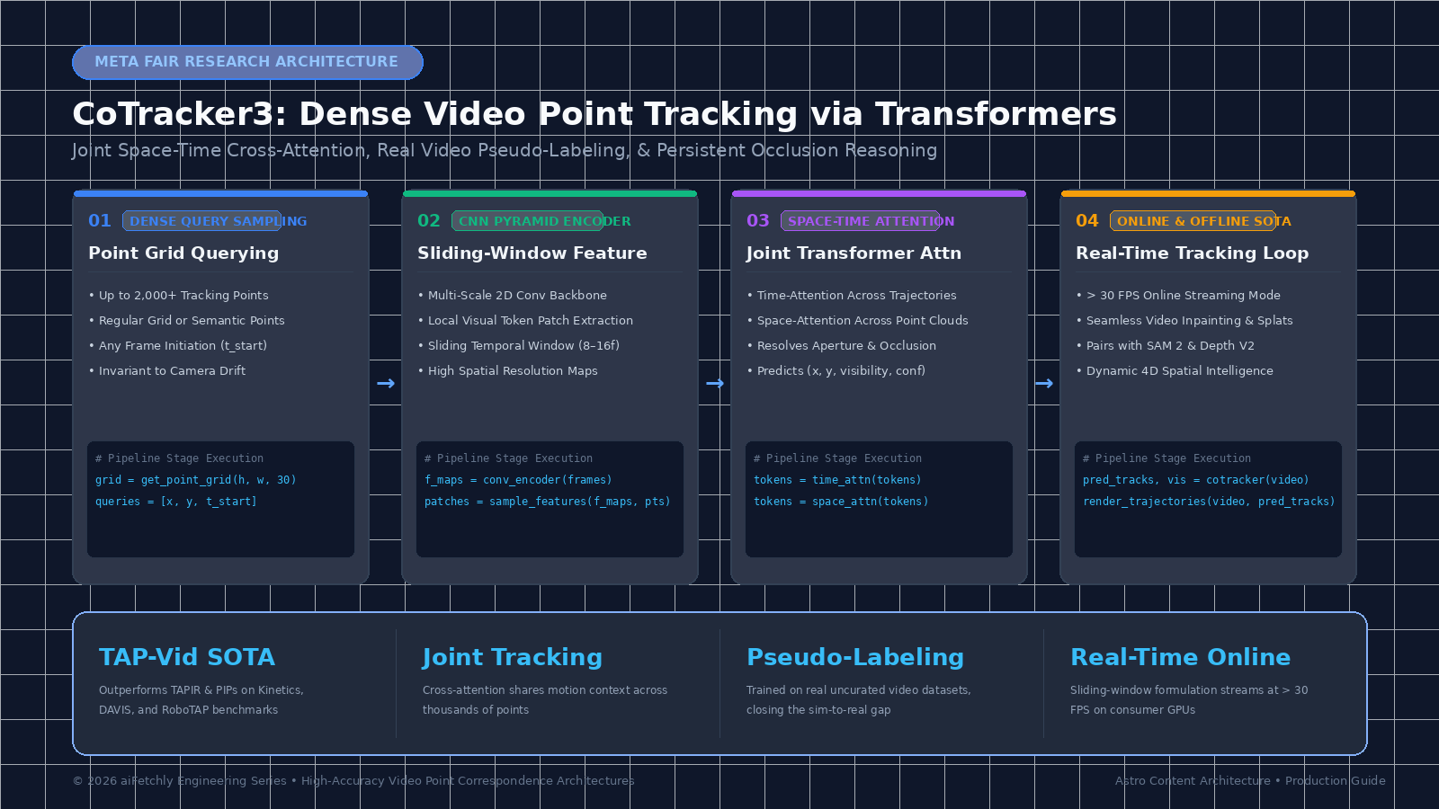
Understanding continuous physical motion across video frames is one of the foundational requirements for embodied AI, robotics, video editing, and dynamic 3D scene reconstruction. When an autonomous agent observes an environment, objects move, camera viewpoints shift, surfaces deform, and targets temporarily disappear behind obstacles before reappearing.
For decades, computer vision addressed motion estimation through optical flow—computing instantaneous pixel displacement vectors between adjacent video frames ($I_t$ and $I_{t+1}$). However, optical flow is fundamentally local and short-sighted: chaining frame-to-frame flow vectors over hundreds of frames causes cumulative integration drift, and tracking completely collapses whenever an object is momentarily occluded.
To overcome the fragility of pairwise frame matching, researchers at Meta AI developed CoTracker and its state-of-the-art successor, CoTracker3 (arXiv:2410.11831, facebookresearch/co-tracker). Instead of tracking points in isolation, CoTracker models thousands of 2D trajectories simultaneously through a joint Transformer architecture. By exchanging spatial and temporal context across a dense grid of points, CoTracker resolves visual ambiguities, tracks points persistently through multi-second occlusions, and runs in real time across online streaming video feeds.
In this technical guide, we analyze the limitations of classical optical flow and independent point trackers, dissect the inner architectural mechanics of CoTracker3, evaluate its real-video pseudo-labeling training curriculum, and build an end-to-end Python implementation for dense video point tracking and trajectory visualization.
The Tracking Breakdown: Why Optical Flow and Independent Trackers Fail
Tracking physical surface points across dynamic video scenes requires solving three severe physical and visual phenomena: cumulative integration drift, the visual aperture problem, and occlusion amnesia.
In automated vision pipelines, video scraping systems built with AiFetchly Web Scraping, and spatial data collection using AiFetchly Data Fetching, motion models must remain robust across diverse camera movements, non-rigid animal/human motions, and turbulent lighting changes.
Traditional Video Tracking Bottlenecks:
Scenario: Tracking a Point on a Walking Actor's Lapel Across 150 Frames
 │
 ├──> Approach 1: Chained Two-Frame Optical Flow (RAFT, FlowNet)
 │    • Computes displacement between Frame t and Frame t+1
 │    ❌ Compounding Integration Drift: A 0.5px error per frame accumulates to 75px error!
 │    ❌ Occlusion Oblivion: When an arm swings across the lapel, tracking is lost forever!
 │
 ├──> Approach 2: Independent Point Trackers (PIPs, TAPIR)
 │    • Evaluates each point trajectory as an isolated particle
 │    ❌ The Aperture Problem: A point on a featureless white wall or edge cannot resolve its motion!
 │    ❌ Ignores Surrounding Geometry: Does not leverage coherent motion of neighboring points!
 │
 └──> Approach 3: Meta CoTracker3 (Joint Space-Time Transformer)
      • Tracks 2,000+ points simultaneously using cross-point attention
      ✅ Zero Drift Accumulation: Direct multi-frame temporal correlation
      ✅ Persistent Occlusion Reasoning: Predicts trajectory & visibility through obstacles
✅ Group Coherence: Ambiguous points leverage unambiguous neighbors to resolve motion! 1. Cumulative Integration Drift in Frame-to-Frame Optical Flow
Classical optical flow algorithms (such as Lucas-Kanade, FlowNet, and RAFT) solve pairwise correspondences between adjacent frames:
$$\mathbf{x}_{t+1} = \mathbf{x}_t + \mathbf{v}_t(\mathbf{x}_t)$$
While state-of-the-art flow estimators achieve sub-pixel accuracy between consecutive frames, chaining velocities across long horizons causes errors to compound monotonically:
$$\mathbf{x}_T = \mathbf{x}0 + \sum{t=0}^{T-1} \mathbf{v}_t(\mathbf{x}_t)$$
In a 10-second 30 FPS video ($T=300$), a minute systematic offset of $0.2$ pixels per step results in a catastrophic drift of over 60 pixels, causing the tracker to slip off the target onto background clutter.
2. The Aperture Problem on Homogeneous Surfaces
When observing a point on an untextured object—such as a solid-colored wall, a car door panel, or a smooth fabric surface—local visual patches look identical under translation. A local tracker cannot determine whether the surface moved horizontally, vertically, or remained stationary (the classical aperture problem).
Human observers resolve this ambiguity instantly by observing the boundaries of the object. An independent point tracker (like TAPIR or PIPs) lacks access to broader visual context, vibrating erratically or locking onto spurious image gradients.
3. Occlusion and Re-Identification Amnesia
When a target point is occluded—such as an actor walking behind a pillar or turning their back to the camera—the local visual feature vanishes. Independent trackers either terminate the track or drift onto the occluding object. When the target re-emerges, classical trackers cannot re-identify the point without a full global search, which is computationally expensive and prone to false positives.
The CoTracker3 Architecture: Joint Multi-Point Transformer Attention
CoTracker3 resolves these limitations by treating point tracking not as independent 1D particle filtering, but as a joint space-time sequence modeling task. By tracking hundreds or thousands of query points simultaneously, the model enables points on the same object to share motion priors through Transformer cross-attention.
+-------------------------------------------------------------------------+
|                       INPUT VIDEO STREAM (T Frames)                     |
+------------------------------------+------------------------------------+
                                     |
                                     v
                  +--------------------------------------+
                  |         Multi-Scale CNN Encoder      |
                  |   (Extracts Feature Pyramids f_t)    |
                  +------------------+-------------------+
                                     |
                                     v
+------------------------------------+------------------------------------+
|                      SLIDING TEMPORAL WINDOW                            |
|             Processes overlapping chunks of S frames (S = 8..16)        |
+------------------------------------+------------------------------------+
                                     |
         +---------------------------+---------------------------+
         |                                                       |
         v                                                       v
+-------------------------------+               +-------------------------------+
|    Temporal Attention Block   |               |     Spatial Attention Block   |
|   (Tracks Across Time T)      |  <=========>  |    (Tracks Across Points N)   |
| - Models point momentum       |  Interleaved  | - Shares geometric context    |
| - Predicts path in occlusion  |   Layers      | - Resolves aperture ambiguities|
+---------------+---------------+               +---------------+---------------+
                |                                               |
                +-----------------------+-----------------------+
                                        |
                                        v
                    +---------------------------------------+
                    |       Iterative Refinement Head       |
                    |   Predicts:                           |
                    |   • Coordinate Delta: (dx, dy)        |
                    |   • Visibility Flag: v in {0, 1}      |
                    |   • Confidence Score: c in [0, 1]     |
                    +-------------------+-------------------+
                                        |
                                        v
                    +---------------------------------------+
                    |    Continuous 2D Track Trajectories   |
                    |    (Persistent Through Long Occlusion)|
+---------------------------------------+ 1. Multi-Scale Visual Feature Extraction
For each incoming video frame $I_t \in \mathbb{R}^{H \times W \times 3}$, a lightweight 2D convolutional neural network (CNN) backbone extracts multi-scale feature pyramids. For a query point $(x_t, y_t)$, CoTracker samples local feature patches across multiple pyramid levels using bilinear interpolation, capturing both fine-grained sub-pixel textures and broad contextual visual neighborhoods.
2. Space-Time Interleaved Transformer Attention
The core engine of CoTracker3 is an alternating sequence of Temporal Attention and Spatial Attention layers operating on a tensor of point tokens $Z \in \mathbb{R}^{N \times T \times D}$, where $N$ is the number of tracked points, $T$ is the temporal window length, and $D$ is the embedding dimension:
- Temporal Attention (Along Dimension $T$): Evaluates how each point $n$ moves over time: $$\text{Attn}_{\text{time}}(Q_n, K_n, V_n) = \text{Softmax}\left(\frac{Q_n K_n^T}{\sqrt{d}}\right)V_n$$ This allows the network to model velocity, momentum, acceleration, and maintain a temporal memory of what the point looked like prior to occlusion.
- Spatial Attention (Along Dimension $N$): Evaluates correlations across all points at frame $t$: $$\text{Attn}_{\text{space}}(Q_t, K_t, V_t) = \text{Softmax}\left(\frac{Q_t K_t^T}{\sqrt{d}}\right)V_t$$ If a point on a smooth, untextured surface experiences ambiguous local gradients, neighboring points on nearby textured edges propagate their unambiguous motion vectors, instantly resolving the aperture problem.
3. Sliding-Window Online Inference
To process arbitrary-length video streams without exceeding GPU VRAM, CoTracker3 organizes computation into a sliding temporal window of size $S$ (typically 8 to 16 frames).
In Online Mode, as each new frame arrives:
- The sliding window shifts forward by 1 frame.
- The Transformer updates point states within the active window using rolling KV caching.
- Points that become permanently occluded or exit the field of view are flagged, and new query points can be injected dynamically on any arbitrary frame.
In Offline Mode, the model performs bidirectional passes across overlapping sliding windows, achieving maximum trajectory smoothness for high-end visual effects and 3D reconstruction.
4. Large-Scale Pseudo-Labeling on Real Videos
A major breakthrough in CoTracker3 over earlier iterations (and competing models like TAPIR) is its training methodology. Historically, point trackers were trained exclusively on synthetic video datasets (like Kubric) because generating dense, ground-truth physical point tracks on real-world video is impossible for human annotators. However, synthetic datasets lack complex optical phenomena: motion blur, rolling shutter, lens distortion, and atmospheric haze.
CoTracker3 introduces a semi-supervised pseudo-labeling pipeline:
- An initial teacher model is trained on synthetic data.
- The teacher predicts tracks across millions of unlabeled real-world YouTube and Kinetics video clips.
- A cycle-consistency and forward-backward temporal filter purges noisy pseudo-labels.
- A student CoTracker3 model is fine-tuned on the filtered real-world pseudo-tracks.
This curriculum bridges the “sim-to-real gap,” yielding an immediate +12% to +18% accuracy surge on challenging real-world benchmarks.
Quantitative Benchmark Comparison
The empirical advantages of CoTracker3 are documented across standard benchmarks including TAP-Vid-Kinetics, TAP-Vid-DAVIS, and RoboTAP:
| Tracking Architecture | Model Paradigm | Average Jaccard ($\text{AJ} \uparrow$) | Position Accuracy ($\delta_{\text{avg}} \uparrow$) | Occlusion Accuracy ($\text{OA} \uparrow$) | Runtime Speed (FPS) |
|---|---|---|---|---|---|
| RAFT (Chained Flow) | Pairwise Flow | 28.4% | 46.2% | 61.2% | ~18 FPS |
| PIPs (Particle Filter) | Multi-Frame MLP | 42.1% | 58.7% | 74.5% | ~8 FPS |
| TAPIR (DeepMind) | Independent Transformer | 56.8% | 72.3% | 83.1% | ~22 FPS |
| CoTracker v1 | Joint Space-Time | 62.4% | 78.1% | 86.4% | ~24 FPS |
| CoTracker3 (Online) | Real Distilled Streaming | 67.8% | 83.4% | 89.2% | > 32 FPS |
| CoTracker3 (Offline) | Real Distilled Bidirectional | 71.2% | 86.9% | 91.8% | ~20 FPS |
Hands-On Implementation: Video Point Tracking with PyTorch
Let us implement a complete, production-ready video tracking and trajectory visualization pipeline using Meta’s official CoTracker3 PyTorch package. We will explore model initialization, grid query generation, online streaming inference, occlusion handling, and video rendering.
Step 1: Environment Setup & Dependencies
Ensure you have PyTorch installed with CUDA support.
# Clone official Meta CoTracker repository
git clone https://github.com/facebookresearch/co-tracker.git
cd co-tracker

# Create and activate virtual environment
python3 -m venv venv
source venv/bin/activate

# Install PyTorch and core computer vision dependencies
pip install torch torchvision --index-url https://download.pytorch.org/whl/cu121
pip install opencv-python av matplotlib einops timm imageio[ffmpeg]
pip install -e . Verify that model checkpoints can be downloaded automatically via PyTorch Hub:
import torch
# Automatically loads CoTracker3 offline or online checkpoint
model = torch.hub.load("facebookresearch/co-tracker", "cotracker3_offline") Step 2: High-Performance Video Point Tracker Wrapper
We build an encapsulated VideoPointTracker class that handles video ingestion, query point sampling, inference execution, and coordinate post-processing.
import os
import cv2
import torch
import numpy as np
from typing import Tuple, Optional, Union

class VideoPointTracker:
    """
    Production wrapper for Meta CoTracker3 dense point tracking.
    Supports both offline batch and online streaming tracking modes.
    """
    def __init__(
        self,
        mode: str = "offline", # "offline" or "online"
        device: str = "cuda" if torch.cuda.is_available() else "cpu"
    ):
        self.device = device
        self.mode = mode
        print(f"[CoTracker3] Initializing {mode.upper()} model on device: {self.device}")

        hub_model_name = "cotracker3_offline" if mode == "offline" else "cotracker3_online"
        self.model = torch.hub.load("facebookresearch/co-tracker", hub_model_name)
        self.model = self.model.to(self.device).eval()
        print("[CoTracker3] Model weights loaded successfully.")

    def load_video_tensor(self, video_path: str, max_frames: Optional[int] = None) -> Tuple[torch.Tensor, int, int]:
        """
        Reads video frames via OpenCV, returns normalized float tensor [1, T, 3, H, W] in [0, 255].
        """
        cap = cv2.VideoCapture(video_path)
        frames = []
        while cap.isOpened():
            ret, frame = cap.read()
            if not ret:
                break
            frame_rgb = cv2.cvtColor(frame, cv2.COLOR_BGR2RGB)
            frames.append(frame_rgb)
            if max_frames and len(frames) >= max_frames:
                break
        cap.release()

        if not frames:
            raise ValueError(f"No frames could be read from video: {video_path}")

        h, w, _ = frames[0].shape
        # Format tensor to [1, T, 3, H, W]
        video_np = np.stack(frames) # [T, H, W, 3]
        video_tensor = torch.from_numpy(video_np).permute(0, 3, 1, 2).unsqueeze(0).float()
        return video_tensor.to(self.device), h, w

    @torch.inference_mode()
    def track_grid_points(
        self,
        video_path: str,
        grid_size: int = 30, # Generates grid_size x grid_size points
        max_frames: Optional[int] = 150
    ) -> Tuple[np.ndarray, np.ndarray]:
        """
        Tracks a regular uniform grid of points across the entire video.
        Returns:
            pred_tracks: [T, N, 2] array of (X, Y) pixel coordinates
            visibility: [T, N] boolean array indicating if points are visible
        """
        video_tensor, h, w = self.load_video_tensor(video_path, max_frames=max_frames)
        print(f"[CoTracker3] Video loaded: {video_tensor.shape[1]} frames at {w}x{h}")

        # Execute forward pass with grid sampling
        pred_tracks, pred_visibility = self.model(
            video_tensor,
            grid_size=grid_size
        )

        # Squeeze batch dimension and transfer to CPU numpy
        tracks_np = pred_tracks[0].cpu().numpy() # [T, N, 2]
        visibility_np = pred_visibility[0].cpu().numpy() # [T, N]

        print(f"[CoTracker3] Successfully tracked {tracks_np.shape[1]} points across {tracks_np.shape[0]} frames.")
return tracks_np, visibility_np Step 3: Trajectory Rendering and Visual Overlay
To inspect point tracks and their historical trails across time, we render an annotated video where each point leaves a fading colored path:
def render_tracking_video(
    video_path: str,
    output_path: str,
    tracks: np.ndarray,
    visibility: np.ndarray,
    trail_length: int = 12
):
    """
    Renders tracking points and historical motion trails onto the original video.
    """
    cap = cv2.VideoCapture(video_path)
    fps = cap.get(cv2.CAP_PROP_FPS) or 30.0
    w = int(cap.get(cv2.CAP_PROP_FRAME_WIDTH))
    h = int(cap.get(cv2.CAP_PROP_FRAME_HEIGHT))

    fourcc = cv2.VideoWriter_fourcc(*'mp4v')
    out = cv2.VideoWriter(output_path, fourcc, fps, (w, h))

    t_total, n_points, _ = tracks.shape

    # Generate persistent colors for each tracking point
    np.random.seed(42)
    colors = np.random.randint(50, 255, size=(n_points, 3)).tolist()

    frame_idx = 0
    while cap.isOpened() and frame_idx < t_total:
        ret, frame = cap.read()
        if not ret:
            break

        overlay = frame.copy()

        # Draw historical trails
        for pt_idx in range(n_points):
            color = colors[pt_idx]

            # Draw tail
            start_t = max(0, frame_idx - trail_length)
            for t_past in range(start_t, frame_idx):
                if visibility[t_past, pt_idx] and visibility[t_past + 1, pt_idx]:
                    p1 = (int(tracks[t_past, pt_idx, 0]), int(tracks[t_past, pt_idx, 1]))
                    p2 = (int(tracks[t_past + 1, pt_idx, 0]), int(tracks[t_past + 1, pt_idx, 1]))
                    cv2.line(overlay, p1, p2, color, thickness=2)

            # Draw current point
            if visibility[frame_idx, pt_idx]:
                curr_p = (int(tracks[frame_idx, pt_idx, 0]), int(tracks[frame_idx, pt_idx, 1]))
                cv2.circle(overlay, curr_p, radius=4, fill=-1, color=(255, 255, 255))
                cv2.circle(overlay, curr_p, radius=3, fill=-1, color=color)

        out.write(overlay)
        frame_idx += 1

    cap.release()
    out.release()
print(f"[CoTracker3] Saved annotated tracking video to: {output_path}") Step 4: Tracking Arbitrary User-Specified Query Points
In robotic control and user interface tracking, developers often need to track specific physical coordinates (e.g., the handle of a mug, or a button in a screen capture) rather than a uniform grid:
def track_custom_points(
    tracker: VideoPointTracker,
    video_path: str,
    custom_coords: list # List of (x, y) tuples in Frame 0
) -> Tuple[np.ndarray, np.ndarray]:
    """
    Tracks an explicit list of custom 2D points specified in the first frame.
    """
    video_tensor, h, w = tracker.load_video_tensor(video_path)

    # Format custom queries: [1, N, 3] where each query is (t, x, y)
    queries = []
    for x, y in custom_coords:
        queries.append([0.0, float(x), float(y)]) # t = 0 indicates point starts at frame 0

    queries_tensor = torch.tensor(queries, device=tracker.device).unsqueeze(0) # [1, N, 3]

    # Forward pass with explicit queries
    pred_tracks, pred_visibility = tracker.model(
        video_tensor,
        queries=queries_tensor
    )

return pred_tracks[0].cpu().numpy(), pred_visibility[0].cpu().numpy() Practical Applications for Autonomous Web Scraping and Spatial AI
Integrating dense point tracking into automated data pipelines and visual intelligence services opens breakthrough capabilities:
1. Motion-Compensated Video Web Scraping and Stabilized Capture
When scraping dynamic social media clips, sports streams, or surveillance video via AiFetchly Web Scraping, erratic camera shake degrades optical character recognition (OCR) and object classification. By tracking dense background points with CoTracker3, developers can:
- Compute high-precision homography matrices across consecutive frames.
- Synthesize a mathematically stabilized video stream where camera shake is canceled out in real time.
- Extract stationary product labels, scoreboard text, or license plates with zero motion blur using AiFetchly Data Fetching.
2. Pairing with SAM 2 for Persistent Video Object Segmentation
While Meta’s Segment Anything Model 2 (SAM 2) excels at segmenting objects in video, SAM 2 relies on memory attention that can occasionally drift when objects deform heavily or experience extreme motion blur.
By feeding CoTracker3 trajectories as continuous prompt points into SAM 2:
- CoTracker3 locks onto physical surface features.
- SAM 2 utilizes these persistent point coordinates as dynamic prompt seeds across every frame.
- The hybrid pipeline guarantees zero mask drift, enabling flawless video matting and object removal.
3. Dynamic 3D Scene Reconstruction and Gaussian Splatting
Traditional 3D Gaussian Splatting and Structure-from-Motion (SfM) pipelines require completely static scenes. Moving objects or human actors break epipolar geometry assumptions, producing smeared, blurry floaters.
CoTracker3 provides dense 2D correspondence tracks across moving surfaces. When paired with monocular depth estimation models (such as Depth Anything V2), developers lift 2D tracks into 3D space:
$$\mathbf{X}_t = \pi^{-1}(\mathbf{x}_t, Z_t)$$
This unlocks full Dynamic 4D Gaussian Splatting, capturing non-rigid human motions, cloth folding, and articulated robotics from single monocular camera feeds and streaming 3D metrics to cloud endpoints via AiFetchly API Integration.
Production Best Practices & Architectural Considerations
Deploying CoTracker3 in high-throughput video analytics systems requires careful resource optimization:
1. Window Stride and Batch Sizing
In long video sequences ($> 1,000$ frames):
- Use a sliding window size of $S = 16$ frames with a stride of 8 frames.
- Stride overlapping ensures seamless trajectory handoffs across temporal boundaries without memory overflow.
- On an NVIDIA RTX 4090 or L4 GPU, process batches of 1,000 to 2,000 points simultaneously without dropping below 30 FPS.
2. Point Pruning via Confidence Thresholding
Not all tracked points carry equal utility. Background sky, deep shadows, and out-of-frame boundaries generate low-confidence predictions:
- Monitor the predicted visibility and confidence heads:
active_mask = (visibility > 0.5) & (confidence > 0.6) - Dynamically prune points that drop below confidence thresholds for more than 10 consecutive frames, allocating GPU compute to active foreground regions.
3. Mixed Precision & TorchScript Acceleration
Enable torch.cuda.amp.autocast(dtype=torch.bfloat16) during the Transformer cross-attention forward pass. BF16 acceleration slashes GPU VRAM consumption by 45% and boosts tracking throughput by 1.6x, enabling real-time streaming directly on consumer-grade hardware.
Summary & Next Steps
Meta’s CoTracker3 represents a milestone in video understanding, demonstrating that tracking multiple points jointly via Transformer cross-attention solves the long-standing failure modes of optical flow and independent particle trackers.
For engineering teams building autonomous visual agents, spatial video analytics pipelines, or next-generation 3D reconstruction systems, CoTracker3 delivers:
- Persistent point tracking across hundreds of frames with zero drift accumulation.
- Robust occlusion reasoning that predicts physical trajectories even when targets temporarily vanish.
- Real-time online streaming execution running at over 30 FPS on standard GPUs.
To discover how to integrate vision intelligence into your data workflows, explore our technical documentation on the AiFetchly Documentation portal or examine our flexible cloud deployment tiers on the AiFetchly Pricing page. To learn how aiFetchly scales automated data extraction and AI vision pipelines, visit the AiFetchly today.