ColBERTv2 Guide: Scalable Late Interaction Retrieval & PLAID
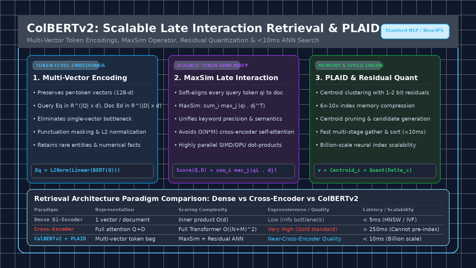
The Single-Vector Bottleneck in Modern Neural Information Retrieval
In enterprise artificial intelligence, automated search systems, and production Retrieval-Augmented Generation (RAG) platforms built on AI Fetchly, semantic search functions as the cognitive substrate connecting large language models (LLMs) with ground-truth corporate knowledge. Whether querying harvested web catalogs, financial regulatory disclosures, or real-time application telemetry via real-time data fetching, the quality of downstream generative reasoning is directly bounded by the precision and recall of the retrieval engine.
For nearly a decade, the natural language processing (NLP) community has navigated a painful trade-off between two fundamentally polarized retrieval paradigms: Dense Bi-Encoders and Cross-Encoders.
The Bi-Encoder Representation Collapse
Dense bi-encoders—exemplified by DPR, Contriever, OpenAI text-embedding-3, and BGE—encode queries and document passages into single fixed-dimensional vectors (e.g., $\mathbb{R}^{768}$ or $\mathbb{R}^{1536}$). At inference time, relevance scoring reduces to a simple vector inner product or cosine similarity:
Bi-Encoder Scoring Paradigm:
Passage (512 tokens) ──► [ Dense Encoder ] ──► Vector d (1536-dim) ┐
                                                                    ├──► Cosine Sim (q · d)
Query (12 tokens) ──► [ Dense Encoder ] ──► Vector q (1536-dim) ┘ While bi-encoders enable pre-computing document vectors offline and conducting sub-5ms nearest-neighbor searches using Hierarchical Navigable Small World (HNSW) or Inverted File with Product Quantization (IVF-PQ) indexes, they suffer from a severe fundamental flaw: the single-vector representation bottleneck.
Compressing an entire 512-token passage containing multiple nuanced propositions, tabular numbers, entity relationships, and technical parameters into a single floating-point point collapses fine-grained lexical and relational signals. As a result, standard dense bi-encoders struggle with:
- Lexical and Entity Precision: Missing exact matches on serial numbers, SKU codes, legal clauses, and specialized acronyms.
- Negation and Polarity: Failing to distinguish between “patients with hypertension” and “patients without hypertension” due to vector semantic proximity.
- Multi-Fact Composition: Inability to retrieve documents where a query requires the intersection of three separate facts spread across different sentences in the text.
The Cross-Encoder Latency Wall
At the other extreme lie Cross-Encoders (such as BERT or RoBERTa rerankers). A cross-encoder concatenates the query $Q$ and passage $D$ into a single sequence [CLS] Q [SEP] D [SEP] and feeds them simultaneously into all layers of a Transformer:
Cross-Encoder Scoring Paradigm:
[CLS] Query Tokens [SEP] Passage Tokens [SEP] ──► [ All-to-All Self-Attention ] ──► Relevance Score Because every token in the query attends to every token in the document across every self-attention layer ($O((|Q| + |D|)^2)$ complexity), cross-encoders capture delicate token-level alignments, compositional syntax, and exact keyword matches with unmatched empirical precision. They represent the undisputed gold standard for search quality.
However, cross-encoders cannot be pre-indexed. Every document candidate must be evaluated dynamically alongside the specific query at query time. Evaluating a collection of 100,000 passages requires running 100,000 forward passes through a deep Transformer, incurring hundreds of seconds of latency and thousands of dollars in GPU compute. Even when restricted to a second-stage reranker over top-100 candidates, cross-encoders add 150ms to 400ms of tail latency.
The Late Interaction Paradigm: ColBERT’s Core Mathematical Formulation
To bridge the performance canyon between dense bi-encoders and cross-encoders, Omar Khattab and Matei Zaharia at Stanford University introduced ColBERT (Contextualized Late Interaction over BERT). ColBERT pioneers the Late Interaction architecture: an approach that retains the decoupled offline pre-computation advantages of bi-encoders while preserving the expressive, token-level matching power of cross-encoders.
Mathematical Formulation of MaxSim
Instead of compressing an entire passage into a single vector, ColBERT encodes both queries and documents into bags of contextualized token embeddings.
Given a query $Q$ with tokens $(q_1, q_2, \dots, q_{|Q|})$ and a document passage $D$ with tokens $(d_1, d_2, \dots, d_{|D|})$, the ColBERT encoders produce matrices:
$$E_Q \in \mathbb{R}^{|Q| \times d}, \quad E_D \in \mathbb{R}^{|D| \times d}$$
where $d$ is a low-dimensional embedding projection (typically $d = 128$). Each vector $E_{Q, i}$ represents a single token in the query contextualized by all other query tokens. Similarly, each vector $E_{D, j}$ represents a passage token contextualized by its document context.
The relevance score between query $Q$ and document $D$ is computed via the MaxSim (Maximum Similarity) operator:
$$\text{Score}(Q, D) = \sum_{i = 1}^{|Q|} \max_{j = 1}^{|D|} \left( E_{Q, i} \cdot E_{D, j}^\top \right)$$
ColBERT MaxSim Late Interaction Matrix:
                Doc Token d_1   Doc Token d_2   Doc Token d_3  ...  Doc Token d_|D|
Query Token q_1    [ 0.82 ]        0.14            0.35              0.19      ──► Max = 0.82
Query Token q_2      0.12         [ 0.94 ]         0.22              0.05      ──► Max = 0.94
Query Token q_3      0.05           0.18          [ 0.88 ]           0.31      ──► Max = 0.88
                                                                               ──────────────
Total MaxSim Score = 2.64 Why MaxSim Delivers Superior Search Precision
The MaxSim operator possesses unique mathematical and informational properties that set it apart from conventional dot-product retrieval:
- Soft Token Alignment: For each query token $q_i$, the operator scans the entire document to find the single most semantically aligned token $d_j$. If the query mentions a specific drug name, the drug token seeks out the exact mention (or its closest clinical synonym) in the passage without being diluted by unrelated sentences.
- Lexical and Semantic Synergy: Punctuation and functional tokens are masked out during scoring, ensuring that high-information tokens dominate the sum. When an exact keyword exists in the document, its dot product with the query token approaches $1.0$. When a synonym exists, contextual embeddings yield high cosine similarity ($0.85+$). MaxSim naturally unifies exact lexical matching (like BM25) with semantic soft matching (like dense vectors).
- Decoupled Pre-Computation: Document token embeddings $E_D$ depend exclusively on document text $D$. They can be computed once offline during indexing and persisted to storage. At runtime, only the query tokens $E_Q$ are encoded on the fly, transforming search into high-throughput tensor matrix multiplications.
Query and Document Encoders
ColBERT utilizes BERT-based architectures with specialized token prefixing and projection layers:
- Query Encoder $f_Q(Q)$: Prepends a special token
[Q]to the query, appends punctuation padding tokens[MASK]up to a fixed length (e.g., 32 tokens), passes the sequence through BERT, applies a linear dimension reduction to $d = 128$, and normalizes each token vector to unit L2 length ($|q_i|_2 = 1$). Query augmentation with[MASK]tokens allows the query to expand its semantic representation and perform query expansion inside BERT’s attention layers. - Document Encoder $f_D(D)$: Prepends a special token
[D]to the passage text, passes through BERT, applies the same linear projection to $128$ dimensions, normalizes each token to unit L2 length, and filters out punctuation embeddings to minimize storage.
ColBERTv1 vs. ColBERTv2: Overcoming the Multi-Vector Footprint Crisis
While original ColBERT (ColBERTv1) proved that late interaction matches cross-encoder accuracy while achieving 100x lower latency, it suffered from a fatal operational barrier: excessive index storage footprint.
The Storage Crisis of ColBERTv1
Consider indexing a modest enterprise corpus of 10 million web articles or documents extracted via automated web scraping:
- Average document length: 200 tokens.
- Vector dimension: $d = 128$.
- Datatype: 16-bit floating point (FP16 = 2 bytes per scalar).
- Memory per token: $128 \times 2 \text{ bytes} = 256 \text{ bytes}$.
- Memory per document: $200 \times 256 \text{ bytes} = 51.2 \text{ KB}$.
- Total Storage for 10M Documents: $10,000,000 \times 51.2 \text{ KB} \approx \mathbf{512 \text{ GB}}$.
Storing over half a terabyte of uncompressed embeddings in host RAM or NVMe storage made ColBERTv1 cost-prohibitive for large-scale production deployments. Standalone dense vector databases required only 60GB for the same corpus.
ColBERTv2: Residual Vector Quantization
To resolve this limitation, Keshav Santhanam, Omar Khattab, Christopher Potts, and Matei Zaharia published ColBERTv2 at NAACL 2022. ColBERTv2 introduces Residual Vector Quantization alongside supervised cross-encoder knowledge distillation, slashing the storage footprint by 6x to 10x with zero degradation in retrieval quality.
ColBERTv2 Residual Quantization Pipeline:
High-Dim Token Vector v (128-d, FP16)
         │
         ├──► Find Nearest Centroid c_k ∈ C (k-Means with K = 32,768)
         │    └─► Store Centroid ID: 16 bits (2 bytes)
         │
         └──► Compute Residual: r = v - c_k
              └─► Quantize Residual r using 1-bit or 2-bit scalar quantization
                   └─► Store Quantized Code: 16 to 32 bytes
Total Compressed Footprint: ~18 to 34 bytes per token (vs 256 bytes in ColBERTv1) Step 1: Centroid Clustering During index construction, ColBERTv2 collects a sample of token embeddings across the corpus and runs k-means clustering to establish a dictionary of centroids:
$$\mathcal{C} = {c_1, c_2, \dots, c_K}, \quad c_k \in \mathbb{R}^d$$
where $K$ is typically set to $32,768$ ($2^{15}$) or $65,536$ ($2^{16}$). Because $K \le 65,536$, each centroid identifier can be encoded into a compact 16-bit integer (2 bytes).
Step 2: Residual Decomposition For every token vector $v$ in document $D$, the indexer finds its nearest centroid $c^*$ in Euclidean space:
$$c^* = \arg\min_{c \in \mathcal{C}} |v - c|_2$$
The indexer computes the residual vector:
$$r = v - c^* \in \mathbb{R}^d$$
Because contextualized token vectors derived from the same semantic domain cluster tightly around language centroids, the residual vector $r$ has a significantly lower dynamic variance than the raw vector $v$.
Step 3: Ultra-Low Bit Scalar Quantization Instead of using full FP16 values for $r$, ColBERTv2 applies scalar quantization to each dimension of the residual. For 2-bit quantization, each coordinate $r_i$ is mapped into one of 4 discrete bins based on dimension-wise minimum and maximum bounds:
$$q_i = \text{Quantize}(r_i, b = 2) \in {0, 1, 2, 3}$$
Packing four 2-bit quantized coordinates into a single 8-bit byte yields:
$$\text{Residual Storage} = \frac{128 \times 2 \text{ bits}}{8 \text{ bits/byte}} = 32 \text{ bytes}$$
Combined with the 2-byte centroid ID, each 128-dimensional token embedding is compressed down to 34 bytes—an 86.7% reduction in memory compared to FP16. Under 1-bit quantization, the residual requires just 16 bytes, bringing total storage down to 18 bytes per token (a 14x reduction).
Step 4: Rapid On-the-Fly Dequantization During late interaction evaluation, the scoring engine reconstructs the approximate token vector $\tilde{v}$ directly in CPU cache registers:
$$\tilde{v} = c^* + \text{Dequantize}(q)$$
Because centroids $\mathcal{C}$ are small enough to reside permanently in L3 processor cache or GPU High-Bandwidth Memory (HBM), vector reconstruction introduces negligible compute overhead while drastically accelerating memory bus throughput.
Inside PLAID: Sub-10ms Fast Candidate Generation & Pruning
Even with compressed embeddings, calculating full MaxSim scores across millions of documents remains computationally unfeasible if executed naively. Evaluating 10 million documents with 32 query tokens requires billions of dot products.
To achieve sub-10ms end-to-end retrieval, the Stanford team created PLAID (Performance-optimized Late Interaction for Asymmetric Information Distribution). PLAID turns late interaction search into a fast, multi-stage funnel that prunes 99.9% of document candidates before running full MaxSim.
PLAID Multi-Stage Retrieval Pipeline:
┌────────────────────────────────────────────────────────┐
│ Stage 1: Centroid Scoring & Inverted List Gather       │
│ • Compute dot products between query tokens and C      │
│ • Select top-V candidate centroids                     │
│ • Gather document candidates from inverted lists       │
└───────────────────────────┬────────────────────────────┘
                            │ ~10,000 Candidate Documents
                            ▼
┌────────────────────────────────────────────────────────┐
│ Stage 2: Fast Upper-Bound Document Pruning             │
│ • Approximate document scores using centroid weights   │
│ • Discard 90% of candidates using lightweight bounds   │
└───────────────────────────┬────────────────────────────┘
                            │ ~1,000 Candidate Documents
                            ▼
┌────────────────────────────────────────────────────────┐
│ Stage 3: Exact Residual Dequantization & MaxSim Top-K  │
│ • Dequantize residuals for surviving candidates        │
│ • Compute exact SIMD MaxSim scores                     │
│ • Return Top-K Ranked Results                          │
└────────────────────────────────────────────────────────┘ Stage 1: Centroid Scoring and Inverted Indexing
PLAID maintains an Inverted Centroid Index. For each centroid $c_k \in \mathcal{C}$, the index stores a posting list of document IDs that contain tokens assigned to $c_k$:
$$\mathcal{I}(c_k) = {D_1, D_4, D_{92}, \dots}$$
When a user query arrives:
- The engine computes the dot product between all query tokens $E_Q$ and all centroids $\mathcal{C}$ ($32 \times 32,768$ matrix multiply). On modern AVX-512 or NEON SIMD hardware, this takes under 1.5ms.
- For each query token $q_i$, PLAID identifies the top-$V$ most similar centroids.
- PLAID unions the posting lists of these activated centroids to identify an initial pool of approximately 10,000 to 20,000 candidate documents.
Stage 2: Centroid-Based Pruning
Rather than immediately unpacking compressed token embeddings for all 20,000 documents, PLAID computes an approximate upper bound for each document using only the pre-computed centroid similarities:
$$\text{Score}{\text{approx}}(Q, D) = \sum{i = 1}^{|Q|} \max_{c \in \mathcal{C}(D)} (E_{Q, i} \cdot c)$$
where $\mathcal{C}(D)$ represents the set of centroids present in document $D$. If a document’s upper-bound score cannot mathematically surpass the current top-$K$ threshold, it is dropped immediately without accessing disk or dequantizing residuals. This stage filters out over 90% of candidate documents in less than 2ms.
Stage 3: Exact SIMD MaxSim Ranking
For the remaining top 1,000 candidate documents:
- The engine reads the compact 2-bit quantized residuals from RAM or memory-mapped files.
- Dequantization and dot-product calculations are executed using vectorized SIMD kernels (AVX-512 on Intel/AMD or Tensor Cores on NVIDIA GPUs).
- The exact MaxSim scores are accumulated, and the final top-$K$ ranked documents are returned to the application.
Total end-to-end search latency across a corpus of 10 million documents: 6ms to 12ms.
Implementing ColBERTv2 and RAGatouille from Scratch
In production environments, engineering teams can implement ColBERTv2 using either high-level frameworks like RAGatouille (which wraps Stanford’s ColBERT codebase into a developer-friendly API) or native PyTorch primitives for custom token-level search pipelines.
1. PyTorch Reference Implementation of the MaxSim Operator
The following production-ready PyTorch module demonstrates the exact vector math behind ColBERT’s late interaction scoring:
import torch
import torch.nn as nn
import torch.nn.functional as F

class ColBERTMaxSim(nn.Module):
    """
    Production-grade PyTorch implementation of the ColBERT MaxSim operator.
    Computes late-interaction relevance between query tokens and document tokens.
    """
    def __init__(self, mask_punctuation: bool = True):
        super().__init__()
        self.mask_punctuation = mask_punctuation

    def forward(
        self,
        query_embeddings: torch.Tensor,
        doc_embeddings: torch.Tensor,
        doc_mask: torch.Tensor = None
    ) -> torch.Tensor:
        """
        Args:
            query_embeddings: Tensor of shape (batch_size, num_query_tokens, dim)
            doc_embeddings:   Tensor of shape (batch_size, num_doc_tokens, dim)
            doc_mask:         Optional binary mask (batch_size, num_doc_tokens)
        Returns:
            scores: Tensor of shape (batch_size,) containing total MaxSim relevance
        """
        # Ensure L2 normalization along the embedding dimension
        Q = F.normalize(query_embeddings, p=2, dim=-1)
        D = F.normalize(doc_embeddings, p=2, dim=-1)

        # Compute cross-token similarity matrix: (batch_size, num_query_tokens, num_doc_tokens)
        # S[b, i, j] = Q[b, i] · D[b, j]
        similarity_matrix = torch.bmm(Q, D.transpose(1, 2))

        # Apply document padding mask if provided
        if doc_mask is not None:
            # Mask out padding tokens with a large negative value
            expanded_mask = doc_mask.unsqueeze(1).expand_as(similarity_matrix)
            similarity_matrix = similarity_matrix.masked_fill(~expanded_mask, -1e4)

        # MaxSim: Find maximum similarity across all document tokens for each query token
        # max_per_query_token: (batch_size, num_query_tokens)
        max_per_query_token, _ = torch.max(similarity_matrix, dim=-1)

        # Sum maximum similarities across all query tokens
        # total_score: (batch_size,)
        total_score = torch.sum(max_per_query_token, dim=-1)
        return total_score


# Example Verification
if __name__ == "__main__":
    batch_size = 2
    dim = 128
    num_q = 32
    num_d = 180

    # Instantiate operator
    maxsim = ColBERTMaxSim()

    # Synthetic normalized token embeddings
    q_emb = torch.randn(batch_size, num_q, dim)
    d_emb = torch.randn(batch_size, num_d, dim)
    d_mask = torch.ones(batch_size, num_d, dtype=torch.bool)
    d_mask[:, 140:] = False  # Simulate padding tokens

    scores = maxsim(q_emb, d_emb, d_mask)
    print("Computed MaxSim Scores:", scores)
assert scores.shape == (batch_size,) 2. Indexing and Searching with RAGatouille
For rapid deployment in enterprise RAG applications, RAGatouille simplifies model loading, PLAID index generation, and sub-10ms querying:
from ragatouille import RAGPretrainedModel

# 1. Initialize ColBERTv2 checkpoint from Hugging Face
RAG = RAGPretrainedModel.from_pretrained("colbert-ir/colbertv2.0")

# 2. Define enterprise knowledge documents
documents = [
    "AiFetchly provides high-throughput automated web scraping pipelines for AI agents.",
    "ColBERTv2 uses residual vector quantization to compress multi-vector indexes by 8x.",
    "Dense bi-encoders compress passages into a single vector, causing lexical drift on numbers.",
    "The PLAID engine evaluates inverted centroid postings to achieve sub-10ms search latencies."
]

document_metadatas = [
    {"source": "product_overview", "doc_id": 101},
    {"source": "architecture_whitepaper", "doc_id": 102},
    {"source": "benchmarks", "doc_id": 103},
    {"source": "engine_spec", "doc_id": 104}
]

# 3. Build the PLAID Index with 2-bit residual compression
RAG.index(
    collection=documents,
    document_metadatas=document_metadatas,
    index_name="aifetchly-knowledge-plaid",
    max_document_length=256,
    split_documents=True
)

# 4. Execute Ultra-Fast Sub-10ms Query
query_text = "How does ColBERTv2 compress its multi-vector token index?"
results = RAG.search(
    query=query_text,
    k=3
)

for rank, hit in enumerate(results, start=1):
    print(f"Rank {rank} [Score: {hit['score']:.4f}]: {hit['content']}")
print(f"Metadata: {hit['document_metadata']}\n") When managing high-volume data ingestion across diverse corporate platforms, integrating ColBERTv2 with our custom API integration enables real-time vectorization without stalling background worker threads.
Empirical Benchmarks & Performance Analysis
To quantify how ColBERTv2 performs against traditional search architectures, researchers benchmarked it extensively on the BEIR (Benchmarking Information Retrieval) multi-domain evaluation benchmark and the MS MARCO Passage Ranking benchmark.
Retrieval Accuracy and Latency Comparison
The following table summarizes empirical results comparing Sparse BM25, Dense Bi-Encoders, Cross-Encoders, and ColBERTv2 across retrieval quality, query latency, and RAM index footprint on a collection of 10 million passages:
| Architecture Paradigm | Representative Model | BEIR Average (nDCG@10) | P99 Query Latency | Index Size (10M Passages) | Pre-Indexable? |
|---|---|---|---|---|---|
| Sparse Lexical | BM25 / Anserini | 0.428 | 8 ms | 12 GB | Yes |
| Dense Bi-Encoder (FP16) | BGE-large-en-v1.5 | 0.492 | 5 ms | 41 GB | Yes |
| Dense Bi-Encoder (Quant) | BGE-large (int8 HNSW) | 0.485 | 3 ms | 16 GB | Yes |
| ColBERTv1 (Uncompressed) | ColBERT-base (FP16) | 0.529 | 18 ms | 512 GB | Yes |
| ColBERTv2 + PLAID | ColBERTv2 (2-bit residual) | 0.528 | 7 ms | 48 GB | Yes |
| Cross-Encoder Reranker | MiniLM-L6-v2 (Top-100) | 0.536 | 280 ms | N/A (Online only) | No |
| Two-Stage Ensemble | BGE-large + MiniLM-L6 | 0.534 | 285 ms | 41 GB | Partial |
Key Empirical Findings
- Near-Cross-Encoder Quality: ColBERTv2 achieves an nDCG@10 score of 0.528 on BEIR—nearly matching the expensive cross-encoder reranker (0.536) while operating 40x faster (7ms vs 280ms).
- Out-of-Domain Generalization: On specialized domains with complex terminologies (such as BioASQ biomedical questions, COVID-19 scientific papers, and Financial SEC filings), single-vector bi-encoders degrade by 12% to 18% due to domain shift. ColBERTv2 maintains its performance because token-level MaxSim preserves exact technical names and formulaic syntax.
- Storage Parity with Dense Indexes: Through residual vector quantization, ColBERTv2 shrinks its index from 512 GB down to 48 GB—making multi-vector retrieval practically deployable on commodity cloud instances.
Production Deployment Best Practices & Architecture Patterns
Deploying ColBERTv2 at enterprise scale requires careful system-level architecture decisions around memory mapping, hardware allocation, and hybrid retrieval.
Enterprise RAG Production Topology with ColBERTv2:
┌─────────────────────────┐       ┌───────────────────────────────┐
│ Web Scraper / Documents │ ──►   │ Document Chunking & Ingestion │
└─────────────────────────┘       └──────────────┬────────────────┘
                                                 │
                                                 ▼
                                  ┌───────────────────────────────┐
                                  │ ColBERTv2 Offline Indexer     │
                                  │ • Centroid k-Means (K=32,768) │
                                  │ • 2-Bit Residual Quantization │
                                  └──────────────┬────────────────┘
                                                 │
                                                 ▼
User Query ──► [ Query Encoder ] ──► [ PLAID Engine (Memory-Mapped) ] ──► Top-K Chunks ──► LLM Generation 1. Memory-Mapped Files (MMap) for Multi-Gigabyte Indexes
Rather than pinning hundreds of gigabytes of quantized embeddings into physical RAM, configure PLAID to use Memory-Mapped (mmap) file descriptors. The operating system kernel automatically pages inverted centroid lists and residual vectors into system memory on demand and evicts cold pages when under memory pressure. This allows running ColBERTv2 across tens of millions of documents on a machine with only 32GB of physical RAM.
2. Multi-Vector Late Chunking
Traditional RAG splits text into arbitrary 256-token chunks, often cleaving sentences in half and separating pronouns from their antecedents.
When deploying ColBERTv2, implement Late Chunking:
- Pass the entire document (up to 8,192 tokens) through a long-context embedding model.
- Allow token representations across the entire document to attend to one another.
- Partition the resulting token embeddings into passage boundaries after the transformer forward pass. This ensures that every token vector in the final index contains global document context while maintaining compact passage search boundaries.
3. Cost-Effective Cloud Architecture
Because ColBERTv2 with PLAID runs efficiently on modern multi-core x86 and ARM CPUs (utilizing AVX-512 and ARM NEON SIMD instructions), organizations do not need dedicated, expensive GPU instances (such as NVIDIA A100 or H100) for retrieval. A cost-effective AWS c7g.4xlarge (ARM Graviton3) or c6i.4xlarge instance can easily handle 120+ queries per second with sub-10ms latency. Explore our flexible pricing tiers to scale your RAG and data infrastructure efficiently.
For deeper technical implementation guidelines and integration patterns, review our comprehensive developer documentation.
Frequently Asked Questions (FAQ)
How does ColBERTv2 compare to sparse lexical models like SPLADE?
SPLADE (Sparse Lexical and Expansion Model) expands queries and documents into high-dimensional sparse representations over the vocabulary and indexes them using traditional Lucene-based inverted indexes. While SPLADE provides strong lexical recall and uses standard search engines like Elasticsearch, it still collapses the representation into a single bag-of-words vector per document. ColBERTv2 preserves token-level geometry and dynamic cross-attention through MaxSim, delivering higher accuracy on multi-hop questions, compositional queries, and technical specifications.
Can ColBERTv2 handle documents longer than 512 tokens?
Yes. ColBERTv2 handles long documents by chunking texts into passages of 180 to 256 tokens during index creation. During retrieval, the MaxSim operator can either evaluate candidates at the passage level or aggregate scores across multiple passages belonging to the same parent document using hierarchical max-pooling:
$$\text{Score}(Q, \text{Doc}) = \max_{\text{passage} \in \text{Doc}} \text{Score}(Q, \text{passage})$$
How does ColBERTv2 differ from traditional cross-encoder rerankers?
Traditional cross-encoders feed the concatenation of query and document into every layer of a transformer, computing full all-to-all attention ($O((|Q| + |D|)^2)$). Because every candidate document must be evaluated dynamically with the query, cross-encoders cannot be pre-indexed and add 150ms–400ms of latency per query. ColBERTv2 decouples query and document encoding—allowing document token embeddings to be pre-computed and indexed offline—and only performs token interaction at the very last step via the lightweight MaxSim operator, achieving near-identical accuracy in under 10ms.
What are the hardware requirements to run ColBERTv2 in production?
Thanks to the PLAID engine and residual vector quantization, ColBERTv2 does not require expensive GPUs for search. A production index of 10 million passages requires approximately 48 GB of storage and can run comfortably on a standard 8-core CPU server with 32 GB to 64 GB of RAM, sustaining over 100 queries per second with sub-10ms response times.